Brachistochrone

Problem

The brachistochrone is the most famous variational problem.

The system consists of a single phase. There are \(n_x = 3\) state variables (horizontal displacement \(x\), vertical displacement \(y\), velocity \(v\)) and \(n_u = 1\) control variable (the angle of the tangent to the curve \(\theta\)).

The dynamics equations are

$$ \dot x = v \sin \theta, \quad \dot y = v \cos \theta, \quad \dot v = g \cos \theta, \quad g = 9.81 $$

The system has a single integral (the length of the time interval)

$$ \mathbb{I} = \int_{t_0}^{t_f} 1 \, \mathrm{d}t $$

The initial time is fixed \(t_0 = 0\), and the final time \(t_f\) is free and is an optimization variable. The system has boundary conditions

$$ \begin{align*} \boldsymbol{x}_0 &= \left[0,0,0\right]^\mathrm{T}\\ \boldsymbol{x}_f &= \left[2,2,\text{free}\right]^\mathrm{T} \end{align*} $$

At the system level, the objective function is

$$ \begin{equation*} F = \mathbb I \end{equation*} $$

Code

import numpy as np
import sympy as sp
import matplotlib.pyplot as plt
from pockit.optimizer import ipopt
from pockit.lobatto import System, constant_guess

g = 9.81

S = System(0)
P = S.new_phase(3, 1)
x, y, v = P.x
theta, = P.u
P.set_dynamics([v * sp.sin(theta), v * sp.cos(theta), g * sp.cos(theta)])
P.set_integral([1])
P.set_boundary_condition([0, 0, 0], [2, 2, None], 0, None)
P.set_phase_constraint([theta], [-np.pi], [np.pi])
P.set_discretization(10, 8)
S.set_phase([P])
S.set_objective(P.I[0])

v = constant_guess(P)
v, info = ipopt.solve(S, v)
print(info['status_msg'].decode())
print(info['obj_val']) # 0.8243386694213402

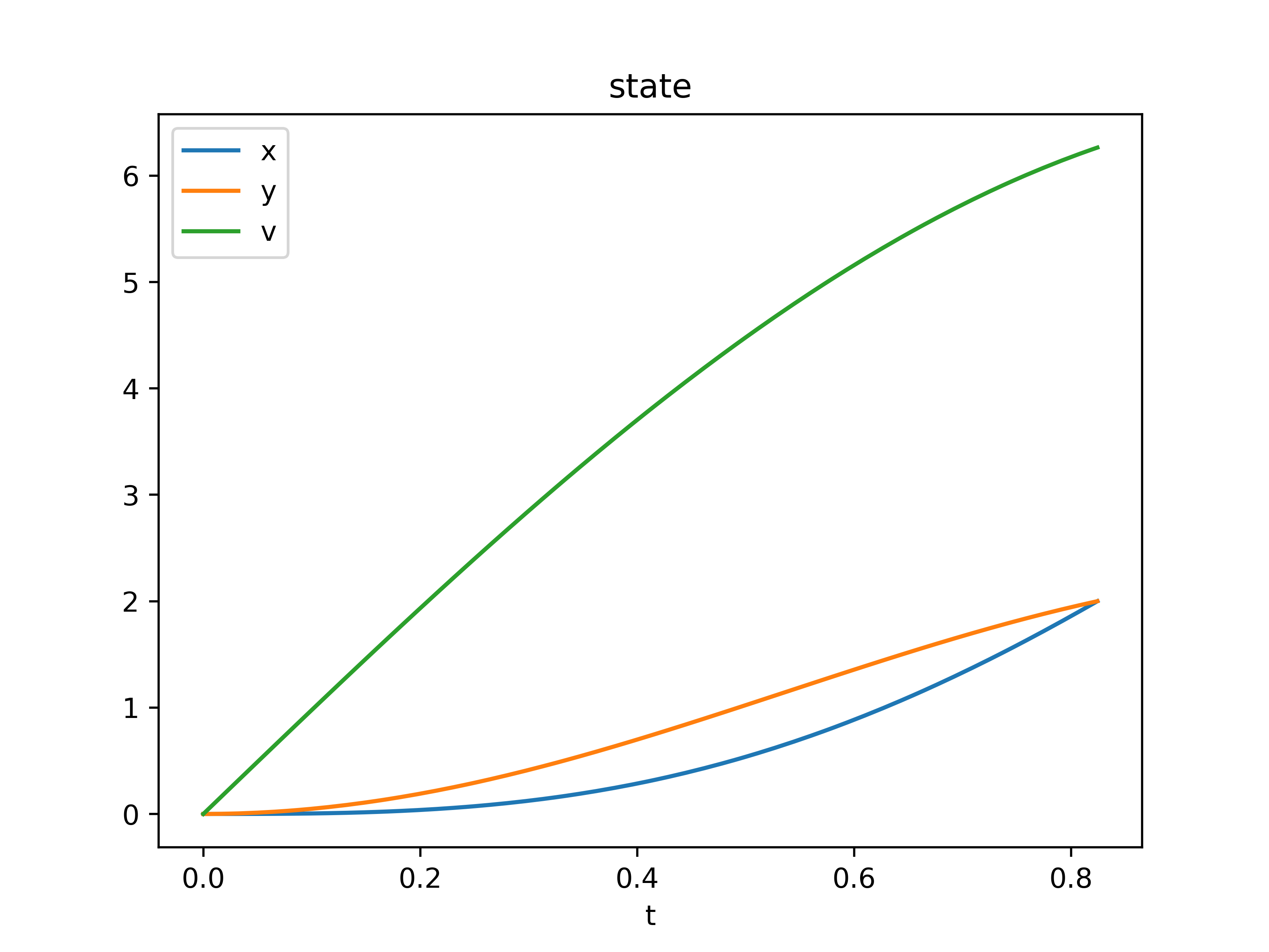
plt.plot(v.t_x, v.x[0])
plt.plot(v.t_x, v.x[1])
plt.plot(v.t_x, v.x[2])
plt.title('state')
plt.legend(['x', 'y', 'v'])
plt.xlabel('t')
plt.show()

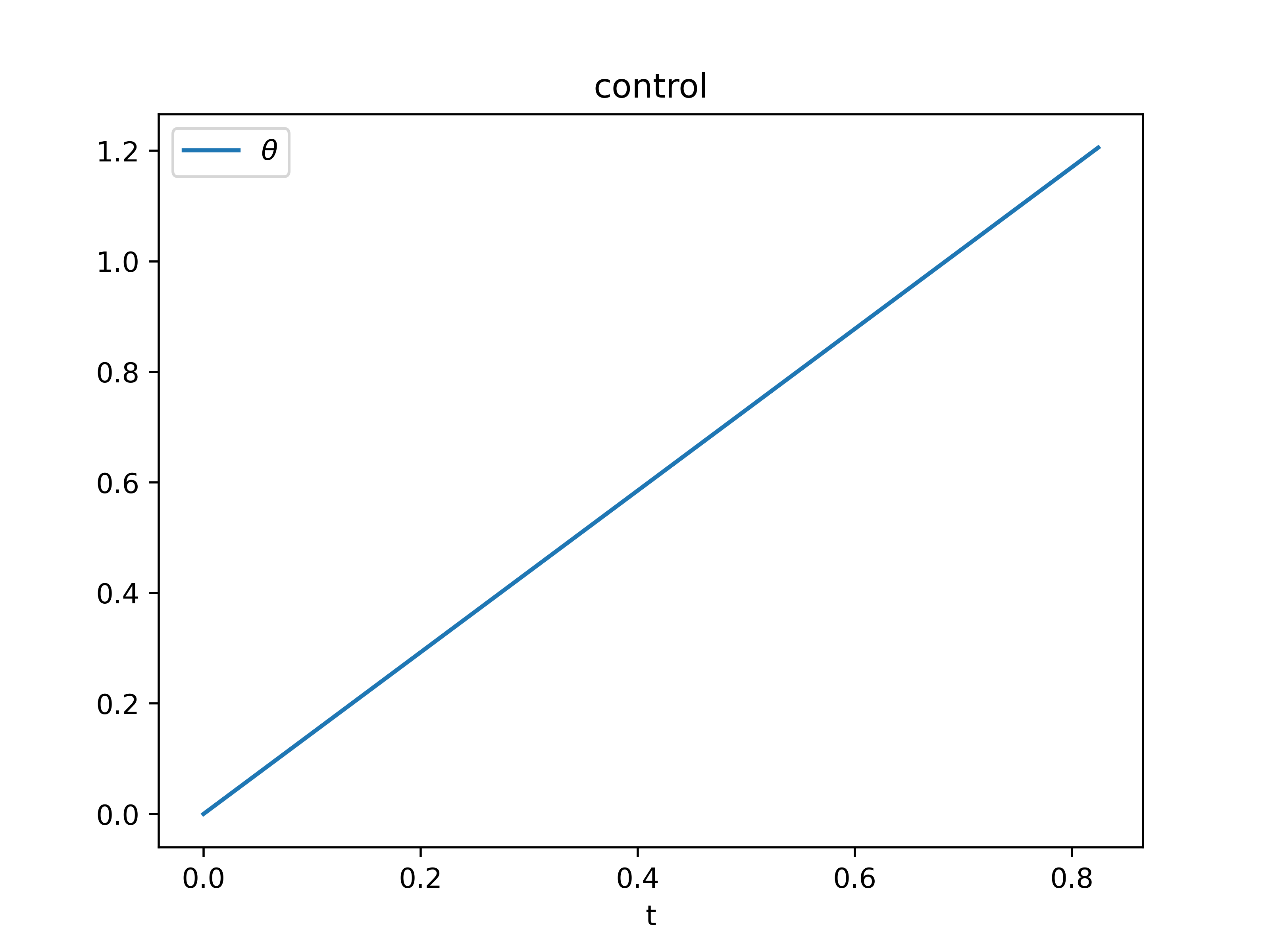
plt.plot(v.t_u, v.u[0])
plt.title('control')
plt.legend([r'$\theta$'])
plt.xlabel('t')
plt.show()

Results