Getting Started

This tutorial introduces pockit's basic workflow through a small optimal-control problem with a known analytical solution. Install pockit first by following the installation guide. The multi-phase problem guide explains the underlying system and phase objects in more detail.

For a compact derivation of the analytical solution and the numerical verification contract, see the double-integrator mathematical reference.

Background

A double integrator models one-dimensional motion when acceleration is the command. Despite its simple dynamics, its minimum-time solution contains a control discontinuity, so it is a useful first test of problem definition, free-time optimization, and result validation.

Pockit replaces the continuous state and control functions with values at collocation nodes. It then transcribes the dynamics, bounds, and objective into a finite-dimensional nonlinear program for a numerical optimizer.

Problem formulation

A unit mass starts one meter from its target at rest. Find the bounded acceleration that brings it to the target, also at rest, in minimum time:

\[ \begin{aligned} \min_{x,v,u,t_f}\quad & t_f = \int_0^{t_f} 1\,\mathrm{d}t \\ \text{subject to}\quad & \dot{x}=v, \qquad \dot{v}=u, \\ & x(0)=1, \quad v(0)=0, \\ & x(t_f)=0, \quad v(t_f)=0, \\ & -1 \le u(t) \le 1. \end{aligned} \]

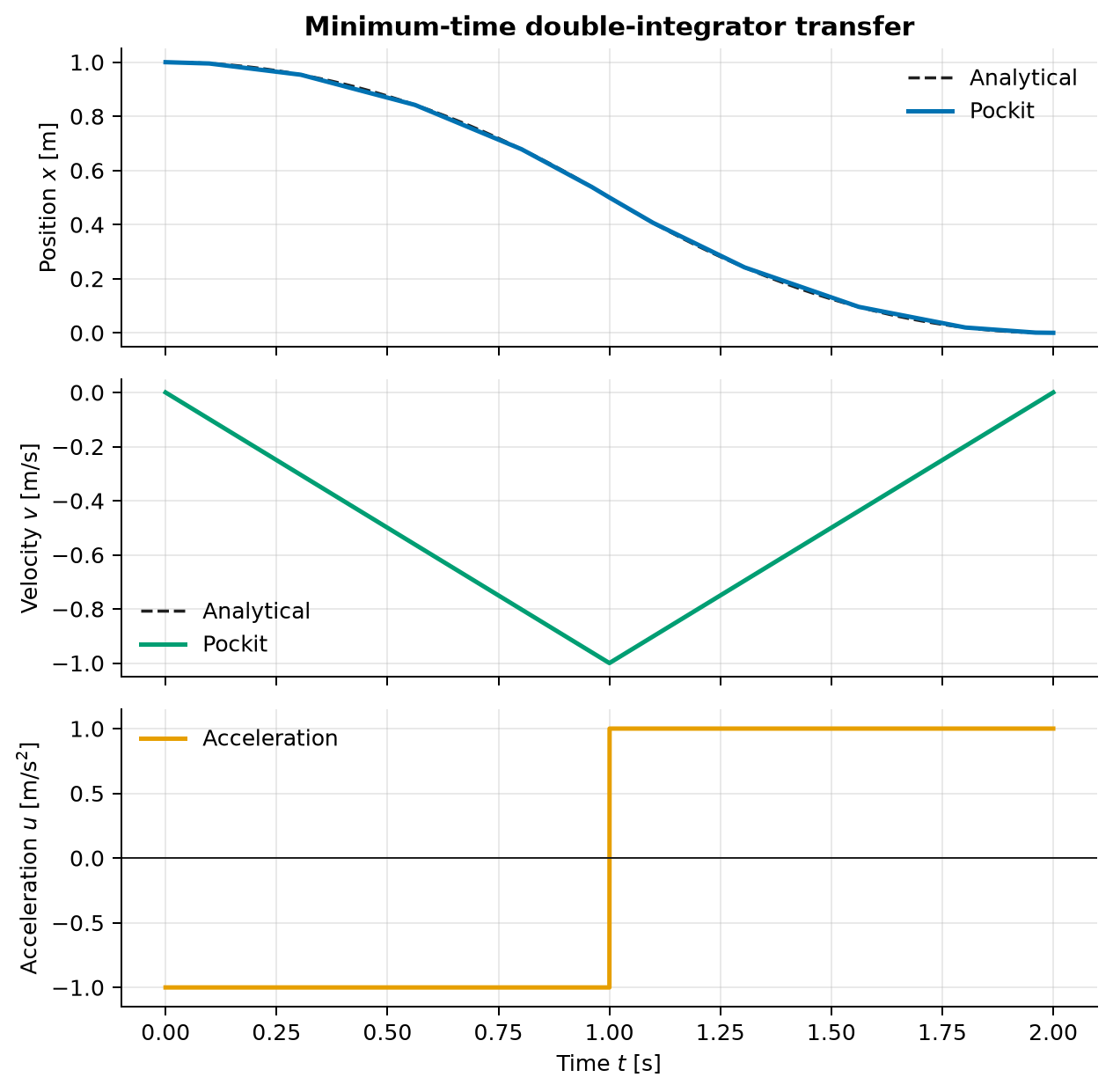
The analytical optimum accelerates toward the target with \(u=-1\), switches at \(t=1\), and brakes with \(u=1\). Therefore \(t_f=2\).

Variables and units

Symbol	Meaning	Unit
\(t\)	Time	s
\(x\)	Position relative to the target	m
\(v\)	Velocity	m/s
\(u\)	Acceleration command	m/s\(^2\)
\(t_f\)	Free final time	s

Modeling choices

The implementation uses a Radau phase with two states and one control. Passing None as the final time makes \(t_f\) an optimization variable. The acceleration bound is a path constraint, and the final True flag identifies its bang-bang character. A mesh boundary at normalized time \(0.5\) lets the discontinuity occur between polynomial segments. The collocation bound is tightened by \(10^{-7}\ \mathrm{m/s^2}\); this negligible transcription buffer keeps the interpolated numerical control inside the physical \(\lvert u\rvert\le1\) limit despite solver tolerance.

Run the example

From the repository root, run:

python -m examples.double_integrator

For a non-interactive run that writes the figure to disk:

python -m examples.double_integrator --save double-integrator.png --no-show

Key implementation

Define the phase, dynamics, bounds, endpoints, and objective:

from pockit.optimizer import ipopt
from pockit.radau import System, linear_guess

MAX_ACCELERATION = 1.0
COLLOCATION_ACCELERATION_LIMIT = MAX_ACCELERATION - 1.0e-7

system = System(0)
phase = system.new_phase(["position", "velocity"], ["acceleration"])
_, velocity = phase.x
(acceleration,) = phase.u

phase.set_dynamics([velocity, acceleration])
phase.set_integral([1.0])
phase.set_phase_constraint(
    [acceleration],
    [-COLLOCATION_ACCELERATION_LIMIT],
    [COLLOCATION_ACCELERATION_LIMIT],
    True,
)
phase.set_boundary_condition([1.0, 0.0], [0.0, 0.0], 0.0, None)
phase.set_discretization([0.0, 0.5, 1.0], [6, 6])
system.set_phase([phase])
system.set_objective(phase.I[0])

A smooth state guess and a two-arc control guess give the optimizer a physically meaningful starting point:

import numpy as np

guess = linear_guess(phase, 0.0)
guess.t_f = 2.2
tau = guess.t_x / guess.t_f
guess.x[0] = 1.0 - 3.0 * tau**2 + 2.0 * tau**3
guess.x[1] = (-6.0 * tau + 6.0 * tau**2) / guess.t_f
guess.u[0] = np.where(
    guess.t_u < guess.t_f / 2.0,
    -COLLOCATION_ACCELERATION_LIMIT,
    COLLOCATION_ACCELERATION_LIMIT,
)

solution, info = ipopt.solve(system, guess)

The complete example also checks the terminal conditions, final time, signs of both control arcs, and the interpolated acceleration at 10,001 physical times. For problems whose switching locations are unknown, System.check() and System.refine() can update the mesh after a solve.

Verified result

The current example produces a minimum time of \(2.000000100109\ \mathrm{s}\) and an estimated switching time of \(1.000000050055\ \mathrm{s}\). Both agree with the analytical bang-bang solution to numerical tolerance. Across 10,001 dense points, the acceleration lies in \([-0.999999900154,\ 0.999999902382]\ \mathrm{m/s^2}\), inside the physical bound.

Source code

See the complete runnable example: examples/double_integrator.py.