Hyper Sensitive Problem

问题描述

系统仅包含一个阶段。有 \(n_x = 1\) 个状态变量和 \(n_u = 1\) 个控制变量。

动力学方程为

$$ \dot x=-x^3 + u $$

系统有单个积分

$$ \begin{equation*} \mathbb{I} = \int_{t_0}^{t_f} \frac 12 \left(x ^ 2 + u ^ 2\right) \mathrm dt \end{equation*} $$

初始、末端时间固定 \(t_0 = 0, t_f=10000\)。系统有边界条件

$$ \begin{align*} \boldsymbol{x}_0 &= \left[3/2\right]^\mathrm{T}\\ \boldsymbol{x}_f &= \left[1\right]^\mathrm{T} \end{align*} $$

系统层面，有目标函数

$$ F = \mathbb I $$

计算程序

import numpy as np
import sympy as sp
import matplotlib.pyplot as plt
from pockit.optimizer import ipopt
from pockit.lobatto import System, linear_guess

S = System(0)
P = S.new_phase(1, 1)
x = P.x[0]
u = P.u[0]
P.set_dynamics([-x ** 3 + u])
P.set_integral([(x ** 2 + u ** 2) / 2])
P.set_boundary_condition([1.5], [1], 0, 10000)
P.set_discretization(10, 10)
S.set_phase([P])
S.set_objective(P.I[0])

v = linear_guess(P)
v, info = ipopt.solve(S, v)
assert info['status'] == 0

max_iter = 20
for i in range(max_iter):
    v, info = ipopt.solve(S, v)
    assert info['status'] == 0
    print("iteration: {}, objective: {}".format(i, info['obj_val']))
    if S.check(v, tolerance_mesh=1e-8):
        break
    v = S.refine(v, num_point_min=10, num_point_max=20, mesh_length_min=1e-8)

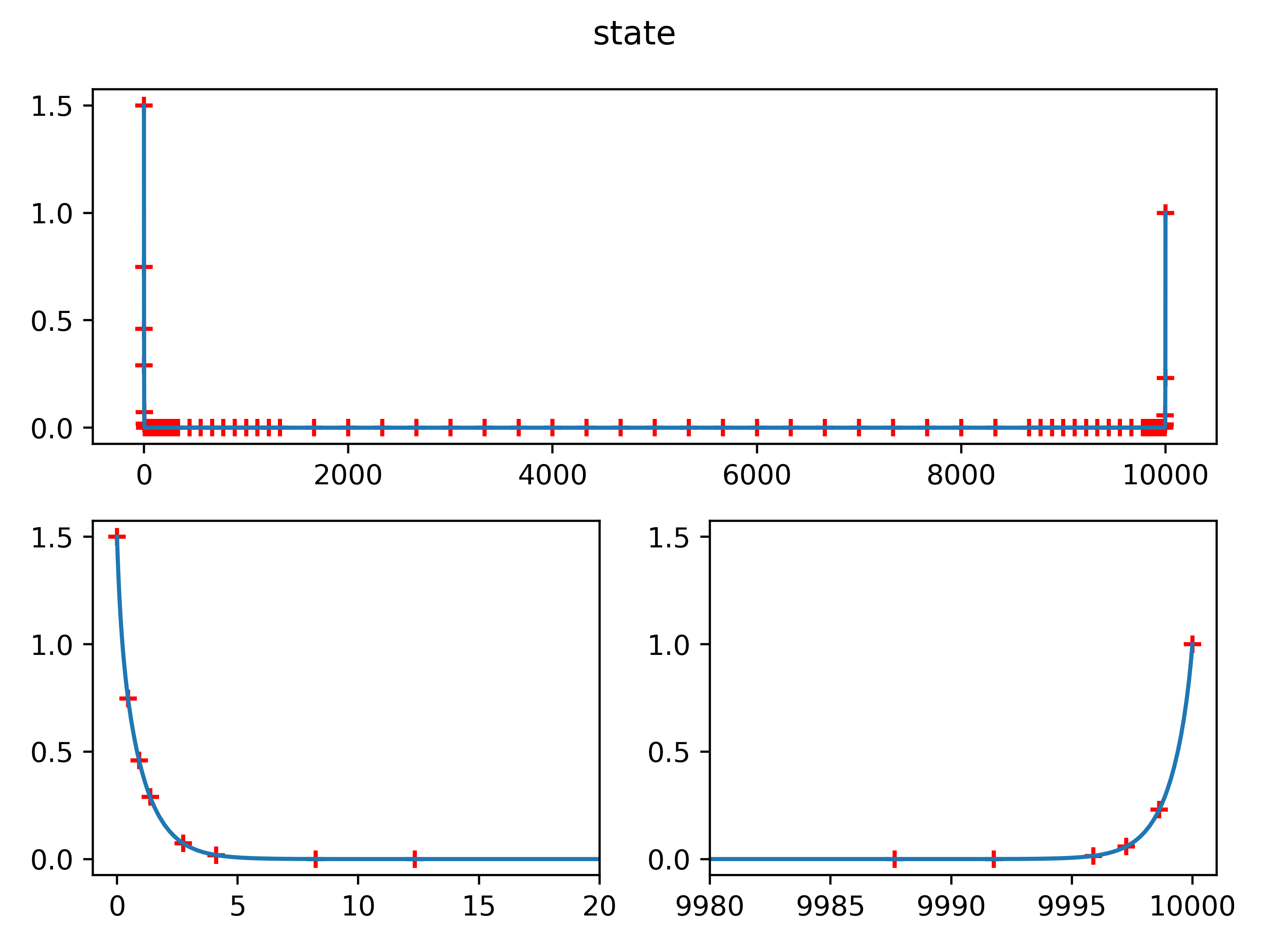
plt.subplot(2, 2, (1, 2))
plt.plot(v.t_x, v.x[0])
plt.scatter(v.t_x[P.l_m], v.x[0][P.l_m], marker='+', s=40, c='r')
plt.scatter(v.t_x[-1], v.x[0][-1], marker='+', s=40, c='r')
plt.subplot(2, 2, 3)
plt.plot(v.t_x, v.x[0])
plt.scatter(v.t_x[P.l_m], v.x[0][P.l_m], marker='+', s=40, c='r')
plt.scatter(v.t_x[-1], v.x[0][-1], marker='+', s=40, c='r')
plt.xlim([-1, 20])
plt.subplot(2, 2, 4)
plt.plot(v.t_x, v.x[0])
plt.scatter(v.t_x[P.l_m], v.x[0][P.l_m], marker='+', s=40, c='r')
plt.scatter(v.t_x[-1], v.x[0][-1], marker='+', s=40, c='r')
plt.xlim([9980, 10001])
plt.suptitle('state')
plt.tight_layout()
plt.show() # '+' denotes mesh point

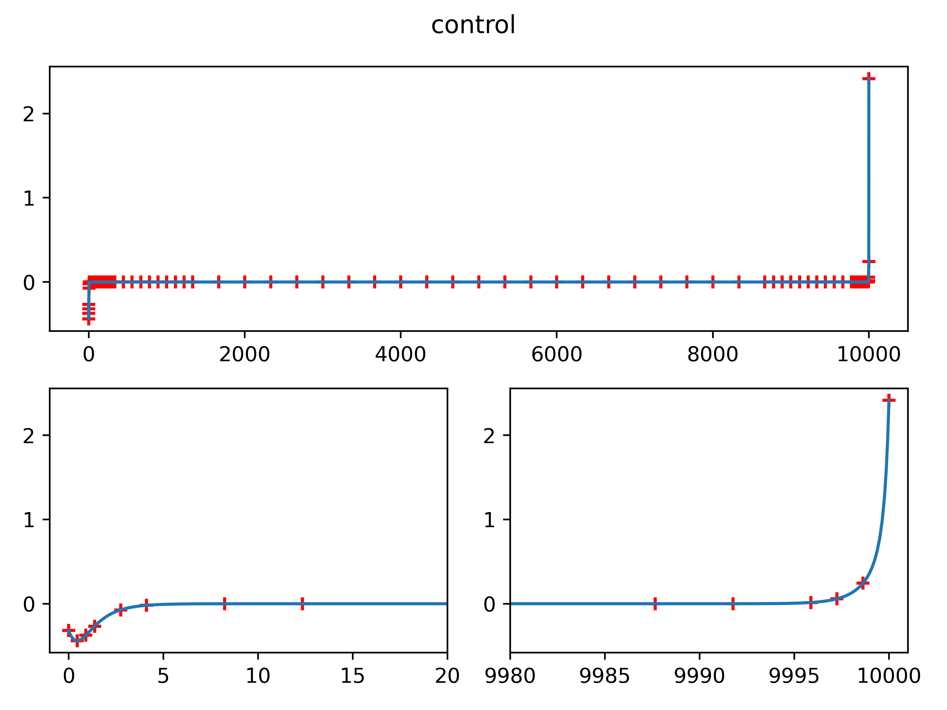
plt.subplot(2, 2, (1, 2))
plt.plot(v.t_u, v.u[0])
plt.scatter(v.t_u[P.l_m], v.u[0][P.l_m], marker='+', s=40, c='r')
plt.scatter(v.t_u[-1], v.u[0][-1], marker='+', s=40, c='r')
plt.subplot(2, 2, 3)
plt.plot(v.t_u, v.u[0])
plt.scatter(v.t_u[P.l_m], v.u[0][P.l_m], marker='+', s=40, c='r')
plt.scatter(v.t_u[-1], v.u[0][-1], marker='+', s=40, c='r')
plt.xlim([-1, 20])
plt.subplot(2, 2, 4)
plt.plot(v.t_u, v.u[0])
plt.scatter(v.t_u[P.l_m], v.u[0][P.l_m], marker='+', s=40, c='r')
plt.scatter(v.t_u[-1], v.u[0][-1], marker='+', s=40, c='r')
plt.xlim([9980, 10001])
plt.suptitle('control')
plt.tight_layout()
plt.show() # '+' denotes mesh point

计算结果