Hyper-Sensitive Problem

Background

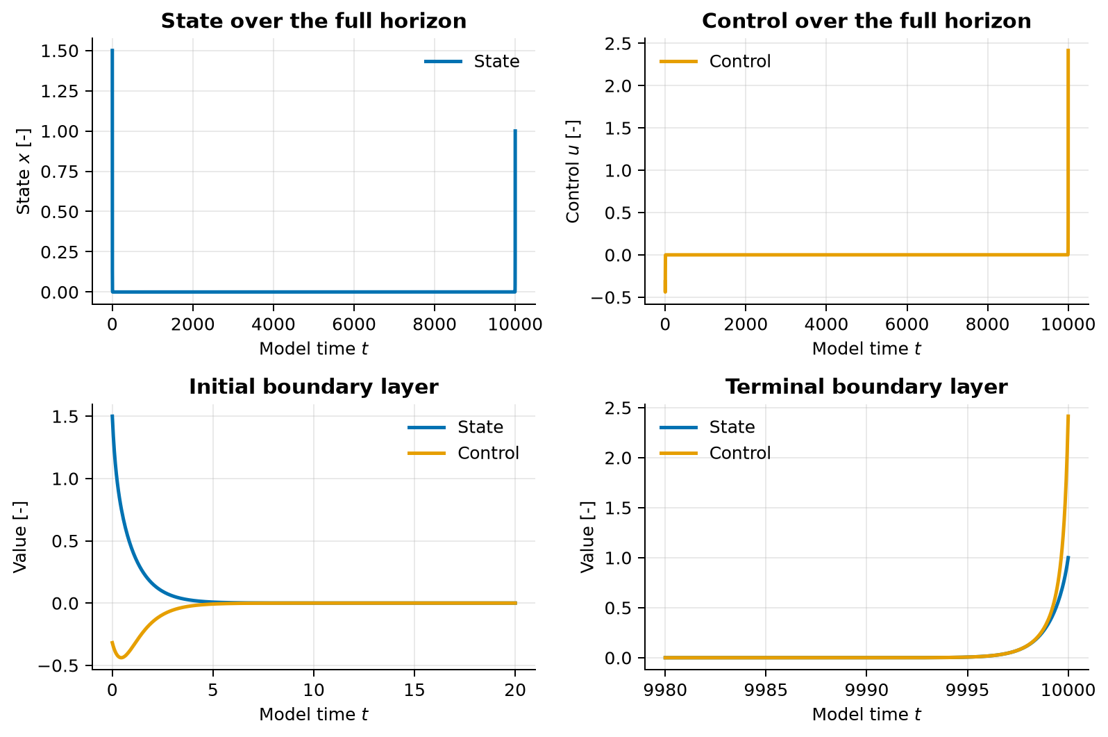
A hyper-sensitive optimal-control problem combines a very long horizon with rapid changes near its endpoints. Most of the trajectory lies close to a slow interior solution, while narrow initial and terminal boundary layers determine whether both endpoint conditions can be met. A uniform fine mesh would spend most of its nodes where little changes.

Problem formulation

The standard scalar benchmark is

\[ \begin{aligned} \min_{x,u}\quad & \frac{1}{2}\int_0^{10000}\left(x^2+u^2\right)\,\mathrm{d}t \\ \text{subject to}\quad & \dot{x}=-x^3+u, \\ & x(0)=1.5, \qquad x(10000)=1. \end{aligned} \]

The quadratic objective penalizes both state magnitude and control effort across the entire horizon.

Variables and units

This benchmark is written entirely in scaled, nondimensional variables. Its model-time horizon is 10,000; assigning seconds without introducing reference scales would make the normalized dynamics dimensionally inconsistent.

Symbol	Meaning	Unit
\(t\)	Model time	-
\(x\)	Scalar state	-
\(u\)	Scalar control	-

Modeling choices

The implementation uses a single fixed-time Lobatto phase. Its initial control guess approximately satisfies the dynamics for the slowly varying state guess. After each successful solve, the mesh-error check determines whether another update is required; refinement concentrates resolution near the two boundary layers instead of filling the quiet interior with uniformly spaced nodes.

Run the example

From the repository root, run the full-accuracy example:

python -m examples.hyper_sensitive

This is deliberately a demanding benchmark and can take more than a minute. To save the figure without opening a window:

python -m examples.hyper_sensitive --save hyper-sensitive.png --no-show

For a shorter smoke test with a coarse error tolerance and at most three mesh updates, add --quick. Quick mode demonstrates the workflow but is not the verified result reported below.

Key implementation

import numpy as np

from pockit.lobatto import System, linear_guess
from pockit.optimizer import ipopt

system = System(0)
phase = system.new_phase(["state"], ["control"])
(state,) = phase.x
(control,) = phase.u

phase.set_dynamics([-(state**3) + control])
phase.set_integral([(state**2 + control**2) / 2.0])
phase.set_boundary_condition([1.5], [1.0], 0.0, 10_000.0)
phase.set_discretization(10, 10)
system.set_phase([phase])
system.set_objective(phase.I[0])

guess = linear_guess(phase, 0.0)
state_at_control_nodes = np.interp(guess.t_u, guess.t_x, guess.x[0])
state_slope = (1.0 - 1.5) / 10_000.0
guess.u[0] = state_at_control_nodes**3 + state_slope
solution, info = ipopt.solve(system, guess)
for _ in range(20):
    if system.check(solution, absolute_tolerance_continuous=1e-8,
                    relative_tolerance_continuous=1e-8):
        break
    solution = system.refine(
        solution,
        absolute_tolerance_continuous=1e-8,
        relative_tolerance_continuous=1e-8,
        num_point_min=10,
        num_point_max=20,
        mesh_length_min=1e-8,
    )
    solution, info = ipopt.solve(system, solution)

The dynamics-informed control guess makes \(\dot{x}\) approximately equal to the slope of the linear state guess. Explicit mesh limits then support reliable convergence.

Verified result

The default example reaches an objective of \(1.330806904944\) after 18 mesh updates. The full-horizon plots show an almost stationary interior; the lower panels reveal the rapid initial and terminal transitions that would otherwise be difficult to see.

Source code

See the complete runnable example: examples/hyper_sensitive.py.