卫星小推力轨道转移

问题描述

考虑 2005-10-7 00:00:00 UTC 从地球出发，1000 天至金星的燃料最优小推力轨道转移问题。出发、到达的位置、速度为

变量	数值	单位
\(r_0\)	[-0.9708322, 0.2375844, -1.671055e-6]	AU
\(v_0\)	[-1.598191, 6.081959.443368e-5]	AU/year
\(r_f\)	[-0.3277178, 0.6389172, 2.765929e-2]	AU
\(v_f\)	[-6.598211, -3.412933, 0.3340902]	AU/year

假设卫星发动机有比冲 \(I_{\text{sp}} = 3800\text{ s}\) 以及最大推力 \(T_{\text{max}} = 0.33 \text{ N}\)。

使用春分点轨道坐标 \(\left[p, f, g, h, k, L\right]^\mathrm{T}\)，其与 Kepler 轨道坐标的关系为。

$$ \begin{align*} & p=a\left(1-e^2\right) \\ & f=e \cos (\omega+\Omega) \\ & g=e \sin (\omega+\Omega) \\ & h=\tan (i / 2) \cos {\Omega} \\ & k=\tan (i / 2) \sin {\Omega} \\ & L=\Omega+\omega+\theta \end{align*} $$

问题有单个阶段，\(n_x = 7\) 个状态变量 \(\left[p, f, g, h, k, L, m\right]^\mathrm{T}\) 和 \(n_u = 3\) 个控制变量 \(\left[u_r, u_t, u_n\right]^\mathrm{T}\)（分别表示径向、切向、法向推力）。

有动力学方程

$$ \begin{align*} &\dot{p}=\frac{2 p}{w} \sqrt{\frac{p}{\mu}} a_t\\ &\dot{f}=\sqrt{\frac{p}{\mu}}\left(a_r \sin L+((w+1) \cos L+f) \frac{a_t}{w}-(h \sin L-k \cos L) \frac{g a_n}{w}\right)\\ &\dot{g}=\sqrt{\frac{p}{\mu}}\left(-a_r \cos L+((w+1) \sin L+g) \frac{a_t}{w}+(h \sin L-k \cos L) \frac{f a_n}{w}\right)\\ &\dot{h}=\sqrt{\frac{p}{\mu}} \frac{s^2 a_n}{2 w} \cos L\\ &\dot{k}=\sqrt{\frac{p}{\mu}} \frac{s^2 a_n}{2 w} \sin L\\ &\dot{L}=\sqrt{\mu p}\left(\frac{w}{p}\right)^2+\frac{1}{w} \sqrt{\frac{p}{\mu}}(h \sin L-k \cos L) a_n\\ &\dot{m} = -\frac{T_{\text{max}} u}{I_{\text{sp}} g_0} \end{align*} $$

其中

$$ \begin{align*} &u = \sqrt{u_r^2 + u_t^2 + u_n^2}\\ &a_r = u_r T_{\text{max}} / m\\ &a_t = u_t T_{\text{max}} / m\\ &a_n = u_n T_{\text{max}} / m\\ &w = 1 + f \cos L + g \sin L\\ &s^2 = 1 + h^2 + k^2\\ &g_0 = 9.80665 \text{ m}/\text{s}^2 \end{align*} $$

有单个阶段约束

$$ 0 \leq u = \sqrt{u_r^2 + u_t^2 + u_n^2} \leq 1 $$

和单个积分

$$ \mathbb I = \int_{t_0}^{t_f}u\,\mathrm dt $$

固定 \(t_0 = 0, t_f = 1000 \text{ days}\)。边界条件由出发、到达的位置、速度计算获得。

系统层面，有目标函数

$$ F=\mathbb I $$

计算程序

import numpy as np
import sympy as sp
import matplotlib.pyplot as plt

from pockit.optimizer import ipopt
from pockit.radau import System, linear_guess

kilogram = 1
second = 1 / 86400 / 365.25
day = 1 / 365.25
meter = 1 / 149597870700
newton = kilogram * meter / second ** 2

i_sp = 3800 * second
t_max = 0.33 * newton
m_0 = 1500 * kilogram
g_0 = 9.80665 * meter / second ** 2
mu = 39.476926

r_0 = [9.708322e-1, 2.375844e-1, -1.671055e-6]
v_0 = [-1.598191, 6.081958, 9.443368e-5]
r_f = [-3.277178e-1, 6.389172e-1, 2.765929e-2]
v_f = [-6.598211, -3.412933, 3.340902e-1]

def Des2MEOE(rv):
    r = np.array(rv[:3])
    v = np.array(rv[3:])
    r_norm = np.linalg.norm(r)
    v_norm = np.linalg.norm(v)
    xi = v_norm ** 2 / 2 - mu / r_norm
    a = - mu / 2 / xi
    h = np.cross(r, v)
    h_norm = np.linalg.norm(h)
    p = h_norm ** 2 / mu
    i = np.arccos(h[2] / h_norm)
    Omega = np.arctan2(h[0], -h[1])
    e_norm = np.sqrt(1 - p / a)
    e = np.cross(v, h) / mu - r / r_norm
    ON = np.array([np.cos(Omega), np.sin(Omega), 0])
    omega = np.arccos(np.dot(ON, e) / e_norm)
    if e[2] < 0:
        omega = 2 * np.pi - omega
    theta = np.arccos(np.dot(e, r) / e_norm / r_norm)
    if np.dot(r, v) < 0:
        theta = 2 * np.pi - theta
    p_meoe = a * (1 - e_norm ** 2)
    f_meoe = e_norm * np.cos(omega + Omega)
    g_meoe = e_norm * np.sin(omega + Omega)
    h_meoe = np.tan(i / 2) * np.cos(Omega)
    k_meoe = np.tan(i / 2) * np.sin(Omega)
    L_meoe = (theta + omega + Omega) % (2 * np.pi)
    return np.array([p_meoe, f_meoe, g_meoe, h_meoe, k_meoe, L_meoe])

def MEOE2Des(meoe):
    p, f, g, h, k, L = meoe
    rv = np.empty(6, dtype=np.float64)
    q = 1 + f * np.cos(L) + g * np.sin(L)
    r = p / q
    s_2 = 1 + h ** 2 + k ** 2
    alpha_2 = h ** 2 - k ** 2
    rv[0] = r / s_2 * (np.cos(L) + alpha_2 * np.cos(L) + 2 * h * k * np.sin(L))
    rv[1] = r / s_2 * (np.sin(L) - alpha_2 * np.sin(L) + 2 * h * k * np.cos(L))
    rv[2] = 2 * r / s_2 * (h * np.sin(L) - k * np.cos(L))
    rv[3] = -1 / s_2 * np.sqrt(mu / p) * (
                np.sin(L) + alpha_2 * np.sin(L) - 2 * h * k * np.cos(L) + g - 2 * f * h * k + alpha_2 * g)
    rv[4] = -1 / s_2 * np.sqrt(mu / p) * (
                -np.cos(L) + alpha_2 * np.cos(L) + 2 * h * k * np.sin(L) - f + 2 * g * h * k + alpha_2 * f)
    rv[5] = 2 / s_2 * np.sqrt(mu / p) * (h * np.cos(L) + k * np.sin(L) + f * h + g * k)
    return rv

S = System(0, fastmath=True)
P = S.new_phase(['p', 'f', 'g', 'h', 'k', 'L', 'm'], ['u_r', 'u_t', 'u_n'])
p, f, g, h, k, L, m = P.x
u_r, u_t, u_n = P.u
a_r = u_r * t_max / m
a_t = u_t * t_max / m
a_n = u_n * t_max / m
w = 1 + f * sp.cos(L) + g * sp.sin(L)
s_2 = 1 + h ** 2 + k ** 2
u_norm = sp.sqrt(u_r ** 2 + u_t ** 2 + u_n ** 2)
dot_p = 2 * p / w * sp.sqrt(p / mu) * a_t
dot_f = sp.sqrt(p / mu) * (
            sp.sin(L) * a_r + ((w + 1) * sp.cos(L) + f) * a_t / w - (h * sp.sin(L) - k * sp.cos(L)) * g * a_n / w)
dot_g = sp.sqrt(p / mu) * (
            -sp.cos(L) * a_r + ((w + 1) * sp.sin(L) + g) * a_t / w + (h * sp.sin(L) - k * sp.cos(L)) * f * a_n / w)
dot_h = sp.sqrt(p / mu) * s_2 * a_n / 2 / w * sp.cos(L)
dot_k = sp.sqrt(p / mu) * s_2 * a_n / 2 / w * sp.sin(L)
dot_L = sp.sqrt(mu * p) * (w / p) ** 2 + 1 / w * sp.sqrt(p / mu) * (h * sp.sin(L) - k * sp.cos(L)) * a_n
dot_m = -t_max * u_norm / i_sp / g_0
P.set_dynamics([dot_p, dot_f, dot_g, dot_h, dot_k, dot_L, dot_m])
meoe_0 = Des2MEOE([*r_0, *v_0])
meoe_f = Des2MEOE([*r_f, *v_f])
P.set_boundary_condition([*meoe_0, m_0], [*meoe_f[:5], meoe_f[5] + 2 * np.pi * 3, None], 0, 1000 * day)
P.set_integral([u_norm])
P.set_phase_constraint([u_norm], [0], [1], [True])
P.set_discretization(50, 3)
S.set_phase([P])
S.set_objective(P.I[0])

v = linear_guess(P, 1e-6)
v, info = ipopt.solve(S, v, optimizer_options={'tol': 1e-8, 'acceptable_tol': 1e-18, 'max_iter': 2000})
print(info['status_msg'].decode())

rv = []
for i in range(len(v.t_x)):
    rv.append(MEOE2Des([v.x[0][i], v.x[1][i], v.x[2][i], v.x[3][i], v.x[4][i], v.x[5][i]]))
rv = np.array(rv).T

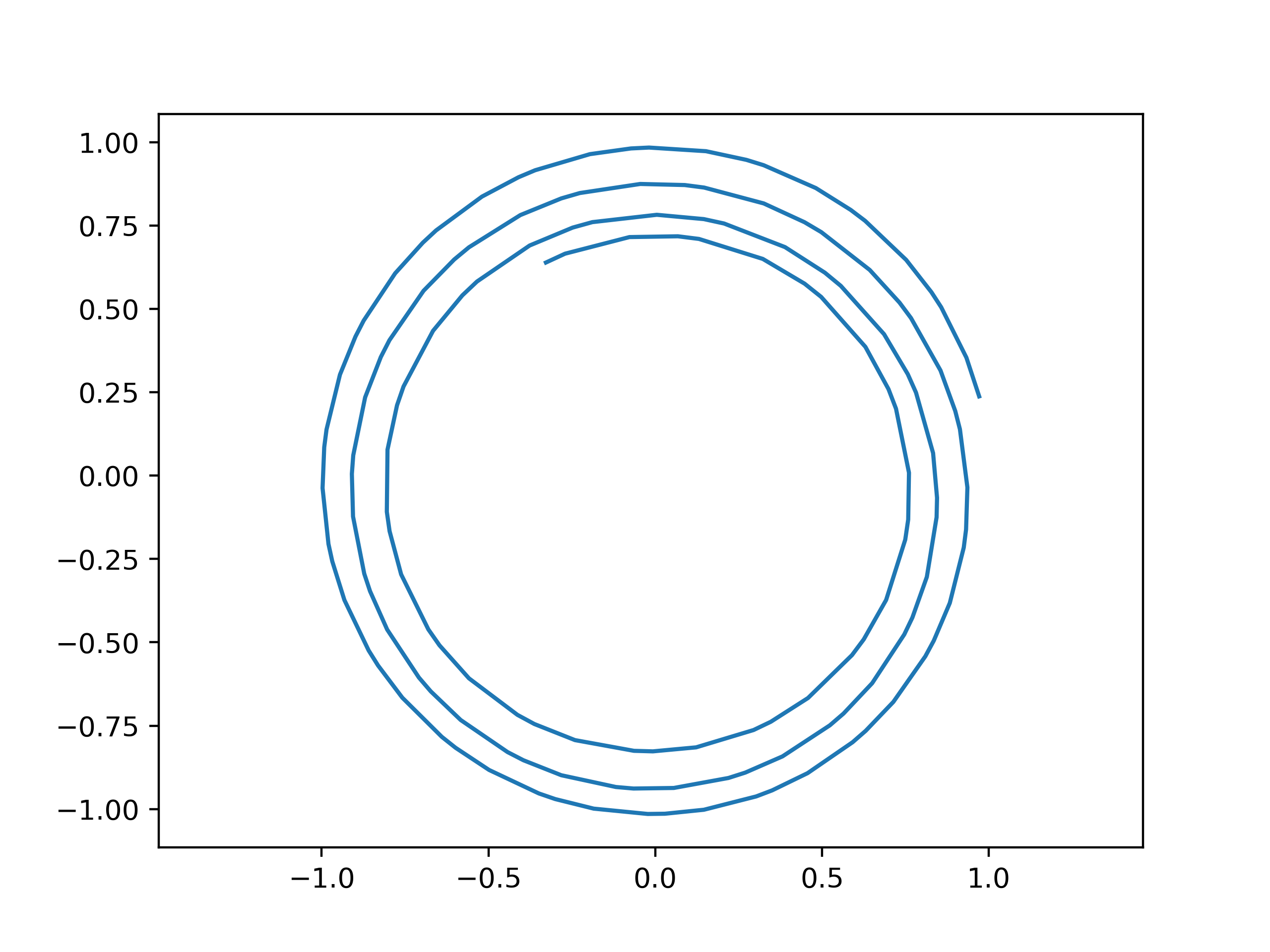
plt.plot(rv[0], rv[1])
plt.axis('equal')
plt.show()

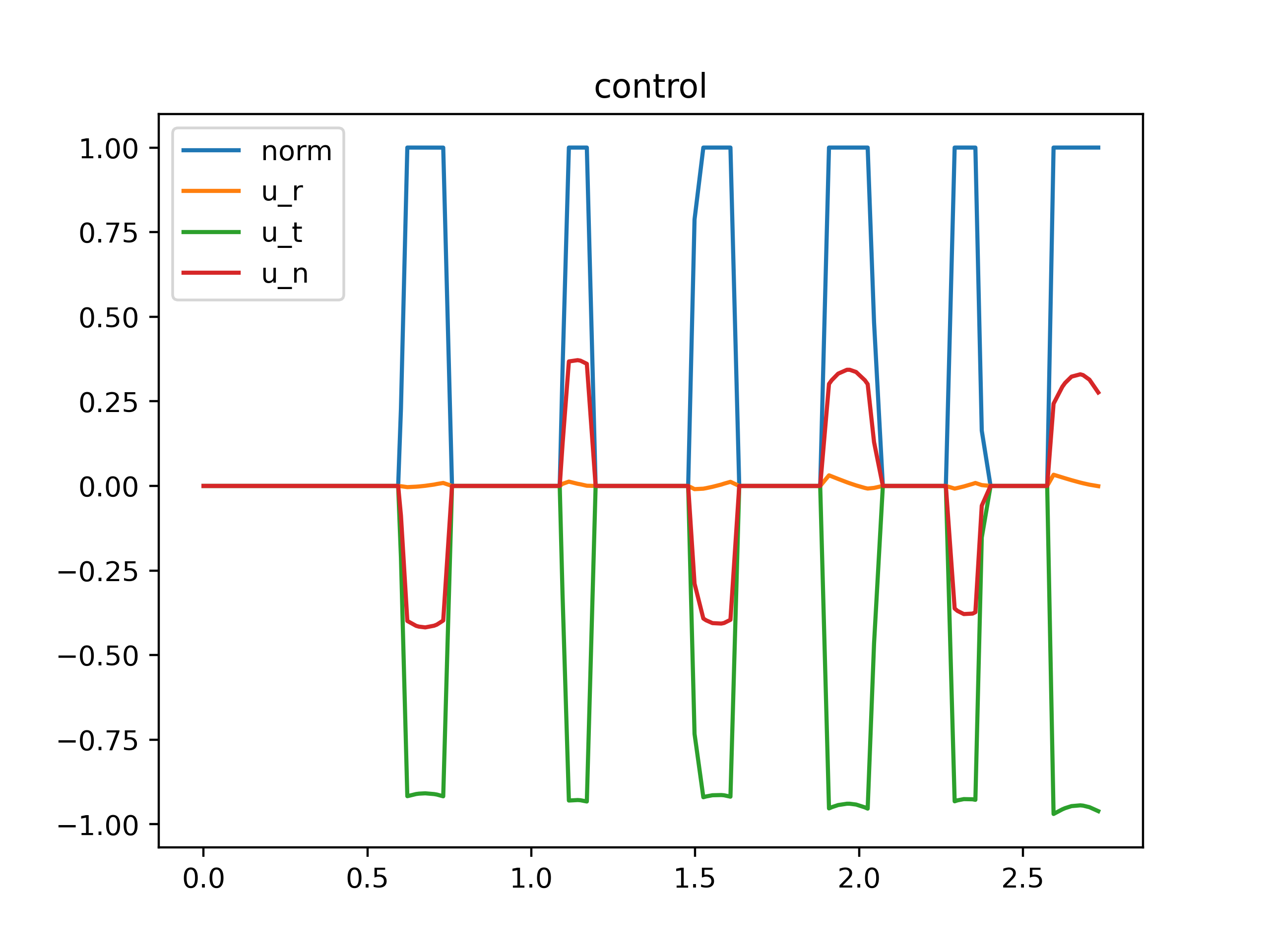
plt.plot(v.t_u, np.sqrt(v.u[0] ** 2 + v.u[1] ** 2 + v.u[2] ** 2), label='norm')
plt.plot(v.t_u, v.u[0], label='u_r')
plt.plot(v.t_u, v.u[1], label='u_t')
plt.plot(v.t_u, v.u[2], label='u_n')
plt.title('control')
plt.legend()
plt.show()

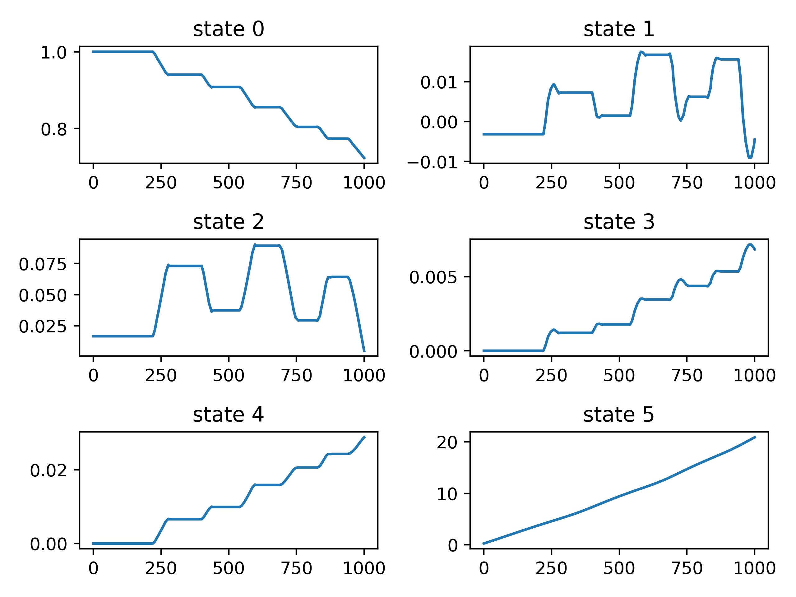
for i in range(6):
    plt.subplot(3, 2, i + 1)
    plt.plot(v.t_x / day, v.x[i])
    plt.title(f'state {i}')
plt.tight_layout()
plt.show()

print(v.x[6][-1] / kilogram) # 1290.554965765408

计算结果