Minimum-Propellant Earth-to-Venus Transfer

Background

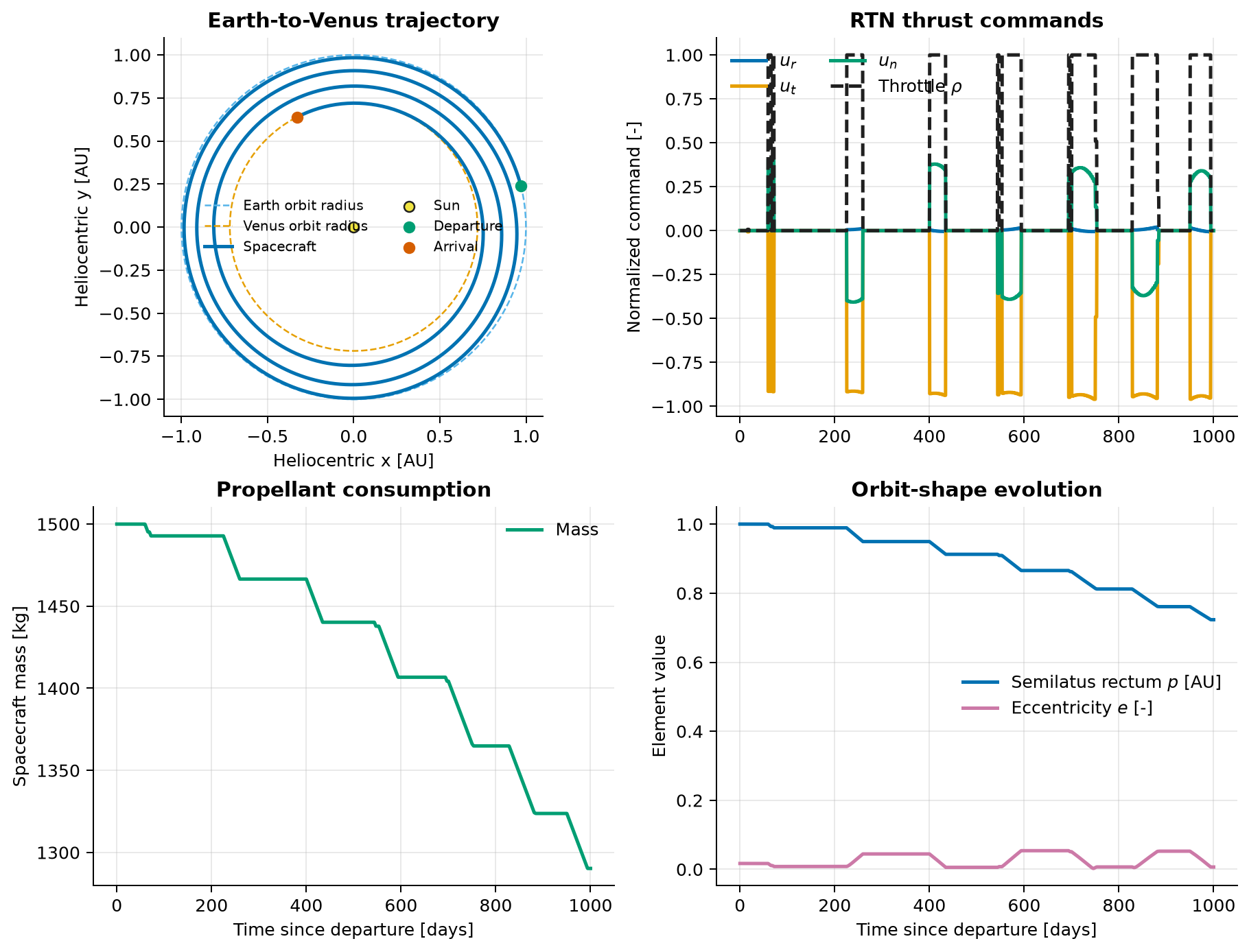
Low-thrust electric propulsion can deliver a large total velocity change while using little propellant, but its small acceleration must act over many months. The thrust direction and throttle therefore have to be planned over the whole trajectory. This example transfers a \(1{,}500\ \mathrm{kg}\) spacecraft from Earth to Venus in exactly 1,000 days and minimizes the consumed propellant.

The heliocentric trajectory is expressed with modified equinoctial elements (MEE). Unlike classical orbital elements, MEE remain regular for circular and equatorial prograde orbits and are well suited to a direct collocation model.

Problem formulation

The heliocentric Cartesian boundary data use astronomical units and Julian years:

Boundary vector	Value	Unit
\(\boldsymbol r_0\)	\([0.9708322,\ 0.2375844,\ -1.671055\times10^{-6}]\)	AU
\(\boldsymbol v_0\)	\([-1.598191,\ 6.081958,\ 9.443368\times10^{-5}]\)	AU/year
\(\boldsymbol r_f\)	\([-0.3277178,\ 0.6389172,\ 2.765929\times10^{-2}]\)	AU
\(\boldsymbol v_f\)	\([-6.598211,\ -3.412933,\ 0.3340902]\)	AU/year

The positive first component of \(\boldsymbol r_0\) is intentional and agrees with Earth's heliocentric longitude on 2005-10-07. A negative sign sometimes shown for this benchmark is inconsistent with the supplied velocity and date.

The state vector and the controls used in the optimization are

\[ \boldsymbol x=[p,f,g,h,k,L,m]^{\mathsf T}, \qquad \boldsymbol q=[d_r,d_t,d_n,\rho]^{\mathsf T}. \]

Here \(p\) is semilatus rectum, \(f,g,h,k\) describe eccentricity and inclination, \(L\) is true longitude, and \(m\) is mass. The vector \(\boldsymbol d=[d_r,d_t,d_n]^{\mathsf T}\) gives a direction inside a protected unit ball, and the nonnegative variable \(\rho\) is the throttle. The physical normalized RTN command is \(\boldsymbol u=\rho\boldsymbol d=[u_r,u_t,u_n]^{\mathsf T}\).

Define

\[ \begin{aligned} w &= 1+f\cos L+g\sin L, & s^2 &= 1+h^2+k^2,\\ \chi &= h\sin L-k\cos L, & \gamma &= \sqrt{\frac{p}{\mu}},\\ [a_r,a_t,a_n]^{\mathsf T} &=\frac{T_{\max}}{m}[u_r,u_t,u_n]^{\mathsf T}. \end{aligned} \]

The MEE and mass dynamics are

\[ \begin{aligned} \dot p &= \frac{2p\gamma}{w}a_t,\\ \dot f &= \gamma\left[ a_r\sin L+\frac{((w+1)\cos L+f)a_t-\chi g a_n}{w}\right],\\ \dot g &= \gamma\left[ -a_r\cos L+\frac{((w+1)\sin L+g)a_t+\chi f a_n}{w}\right],\\ \dot h &= \frac{\gamma s^2\cos L}{2w}a_n,\\ \dot k &= \frac{\gamma s^2\sin L}{2w}a_n,\\ \dot L &= \sqrt{\mu p}\left(\frac{w}{p}\right)^2 +\frac{\gamma\chi}{w}a_n,\\ \dot m &= -c\rho, \qquad c=\frac{T_{\max}}{I_{\mathrm{sp}}g_0}. \end{aligned} \]

The engine parameters are \(T_{\max}=0.33\ \mathrm N\) and \(I_{\mathrm{sp}}=3{,}800\ \mathrm s\). The direction and throttle constraints are

\[ d_r^2+d_t^2+d_n^2\le0.9999^2,\qquad 0\le\rho\le1. \]

Consequently,

\[ u_r^2+u_t^2+u_n^2 =\rho^2(d_r^2+d_t^2+d_n^2) \le0.9999^2\rho^2\le\rho^2. \]

The small relative reserve keeps numerical constraint error inside the physical cone without imposing a positive throttle floor: \(\rho=0\) remains an exact zero-thrust, zero-mass-flow condition.

With fixed initial mass and the same \(\rho\) in the mass equation, minimizing

\[ J=\int_0^{t_f}c\rho\,\mathrm dt=m(0)-m(t_f) \]

is exactly the minimum-propellant objective. The final MEE are fixed to the Venus state, while the final mass is free. The longitude is unwrapped by three complete revolutions so that the collocation trajectory follows the intended continuous branch.

Variables and units

Symbol	Meaning	Unit
\(t\)	Time from departure	Julian year
\(p\)	Semilatus rectum	AU
\(f,g,h,k\)	Equinoctial shape/orientation elements	-
\(L\)	Unwrapped true longitude	rad
\(m\)	Spacecraft mass	kg
\(d_r,d_t,d_n\)	Protected RTN direction vector	-
\(u_r,u_t,u_n\)	Normalized RTN thrust commands	-
\(\rho\)	Engine throttle	-

The script converts the SI values of \(T_{\max}\), \(I_{\mathrm{sp}}\), and \(g_0\) into this AU/year/kg system before constructing the symbolic dynamics.

Modeling choices

The Cartesian-to-MEE conversion is built directly from the angular-momentum and eccentricity vectors. It avoids a chain of inverse cosines, quadrant corrections, and divisions by eccentricity that become fragile near circular orbits. The script checks both boundary states with an MEE-to-Cartesian round trip before solving.

Introducing \(\rho\) separately from \(\boldsymbol d\) is deliberate. Writing mass flow as \(\sqrt{u_r^2+u_t^2+u_n^2}\) is nondifferentiable at zero thrust. The product \(\boldsymbol u=\rho\boldsymbol d\) and the quadratic direction ball are smooth, preserve the interior of the thrust cone, and make the cone apex well behaved: when \(\rho=0\), the physical command is exactly zero regardless of direction.

The solve starts on a \(12\times3\) Radau mesh to obtain a reliable warm start. Both modes then adapt it to 120 one-point Radau intervals. The quick mode stops there; the default mode solves once more on 320 one-point intervals. A one-point Radau control is constant on its interval and its state is linear. Therefore the throttle and direction bounds hold between nodes, and \(\dot m=-c\rho\) makes the interpolated mass nonincreasing. This final low-order representation avoids the unconstrained right-end extrapolation of a high-order Radau control polynomial.

After every final solve, the script evaluates 10,001 evenly spaced times. It raises an explicit exception if throttle leaves \([0,1]\), the physical RTN command leaves the cone, mass increases, or any existing \(p\), \(m\), or \(w\) path bound is violated. The plot uses these validated interpolants; it does not clip an infeasible control.

Run the example

From the repository root, run the verified default solve:

python -m examples.orbit_transfer

Run the reduced final mesh with:

python -m examples.orbit_transfer --quick

To save the default result without opening a window:

python -m examples.orbit_transfer --save orbit-transfer.png --no-show

Key implementation

system = System(0, fastmath=True)
phase = system.new_phase(
    ["p", "f", "g", "h", "k", "longitude", "mass"],
    ["direction_radial", "direction_transverse", "direction_normal", "rho"],
)
d_r, d_t, d_n, rho = phase.u
u_r, u_t, u_n = rho * d_r, rho * d_t, rho * d_n

# The full script defines the six MEE derivatives shown above.
phase.set_dynamics([dot_p, dot_f, dot_g, dot_h, dot_k, dot_L, -c * rho])
phase.set_integral([c * rho])

direction_squared = d_r**2 + d_t**2 + d_n**2
phase.set_phase_constraint(
    [p, mass, w, rho, d_r, d_t, d_n, direction_squared],
    [0.20, 500.0, 0.10, 0.0, -0.9999, -0.9999, -0.9999, 0.0],
    [2.00, 1500.0, np.inf, 1.0, 0.9999, 0.9999, 0.9999, 0.9999**2],
)
phase.set_boundary_condition(
    [*INITIAL_MEE, 1500.0],
    [*TARGET_MEE, None],
    0.0,
    1000.0 / 365.25,
)
phase.set_discretization(12, 3)
system.set_phase([phase])
system.set_objective(phase.I[0])

# After the warm-start solve:
phase.set_discretization(120, 1)  # final quick mesh
# The default mode adapts once more to phase.set_discretization(320, 1).

The complete script contains the coordinate conversions, physical constants, initial spiral guess, staged solves, 10,001-point validation, and plotting.

Verified result

The verified results are:

Mode	Final mesh	Propellant	Final mass
Quick	\(120\times1\)	\(209.872834\ \mathrm{kg}\)	\(1290.127166\ \mathrm{kg}\)
Default	\(320\times1\)	\(209.720375\ \mathrm{kg}\)	\(1290.279625\ \mathrm{kg}\)

For the default solution, all 10,001 samples have \(0\le\rho\le1\). The minimum physical cone margin \(\rho-\lVert\boldsymbol u\rVert_2\) is \(3.162\times10^{-12}\), the minimum quadratic margin is \(5.608\times10^{-23}\), and the maximum direction norm is exactly \(0.9999\) at printed precision. The largest 0.1-day mass change is \(-6.821\times10^{-13}\ \mathrm{kg}\), so no sampled interval gains mass.

The dense semilatus rectum stays in \([0.723300547,1.000381785]\ \mathrm{AU}\), mass stays in \([1290.279625,1500]\ \mathrm{kg}\), and the minimum radius denominator is \(w=0.949954686\). The maximum terminal MEE error is zero at printed precision. On the validation machine, the quick and default commands took about 137 and 157 seconds respectively; compilation caches and hardware affect these timings.

Source code

See the complete runnable example: examples/orbit_transfer.py.