Minimum-Effort Soft Landing on Asteroid Bennu

Background

Landing on a small rotating body is not a scaled-down planetary landing. The gravity is extremely weak, centrifugal acceleration can be comparable to gravity, and a thrust history that looks gentle in inertial space may drift sideways in body-fixed coordinates because of the Coriolis term. Proximity operations therefore benefit from a model expressed in, or consistently transformed to, the rotating surface frame.

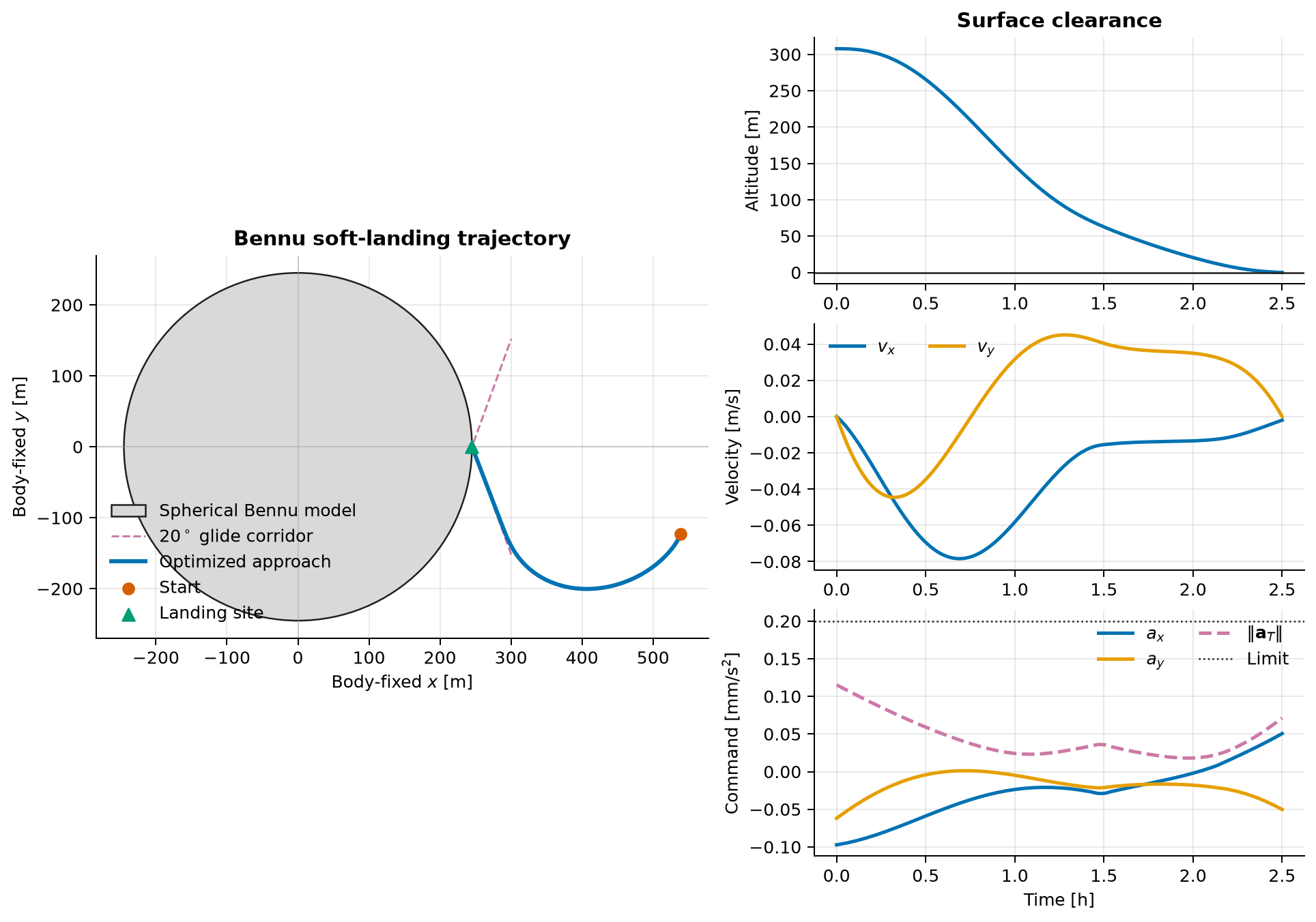
This example plans a planar descent to an equatorial site on asteroid (101955) Bennu. It starts from a nearby point with zero body-relative velocity and reaches first surface contact after \(2.5\) hours with a prescribed inward normal speed of \(2\ \mathrm{mm/s}\). The finite contact speed makes the event unambiguous and directly testable: the pre-contact trajectory must stay outside the body, while the terminal velocity must have the specified small inward component. It is a soft-landing boundary condition, not a zero-velocity rendezvous condition.

This is fundamentally different from the Earth-to-Venus example. Here the motion covers hundreds of meters in an asteroid-fixed rotating frame and must respect a local surface-approach corridor; it is not a heliocentric orbit transfer between planets.

Bennu data and mission assumptions

The spherical model uses rounded early-mission estimates published by the OSIRIS-REx investigation in 2019. They are not presented as the current best-fit values. Rounding is intentional: the example is reproducible, but does not imply that a spherical field represents Bennu's measured irregular shape or full gravity covariance.

Bennu quantity	Symbol	Value
Mean radius	\(R\)	\(245.03\ \mathrm{m}\)
Gravitational parameter	\(\mu\)	\(4.892\ \mathrm{m^3/s^2}\)
Sidereal rotation period	\(P\)	\(4.296057\ \mathrm{h}\)
Rotation rate	\(\omega=2\pi/P\)	\(4.063\times10^{-4}\ \mathrm{rad/s}\)

The following values are transparent design choices for this demonstration; they are not properties of Bennu or a claim about a flown spacecraft.

Mission quantity	Value
Flight time \(T\)	\(9{,}000\ \mathrm{s}=2.5\ \mathrm{h}\)
Maximum commanded acceleration \(a_{\max}\)	\(2.0\times10^{-4}\ \mathrm{m/s^2}\)
Required glide-slope angle \(\gamma\)	\(20^\circ\)
Inward normal contact speed \(v_c\)	\(2.0\times10^{-3}\ \mathrm{m/s}\)

Rotating-frame dynamics

Let the origin be Bennu's center of mass. The \(x\)-axis passes through the target site, the \(y\)-axis lies in the equatorial plane, and the frame rotates at constant angular velocity \(\boldsymbol\Omega=\omega\boldsymbol e_z\). The planar state and commanded thrust acceleration are

\[ \boldsymbol r=(x,y)^{\mathsf T},\qquad \boldsymbol v=(v_x,v_y)^{\mathsf T},\qquad \boldsymbol a_T=(a_x,a_y)^{\mathsf T}. \]

With a spherical gravitational potential, the body-fixed equations are

\[ \dot{\boldsymbol r}=\boldsymbol v, \]

\[ \dot{\boldsymbol v} =-\frac{\mu}{\lVert\boldsymbol r\rVert^3}\boldsymbol r -2\boldsymbol\Omega\times\boldsymbol v -\boldsymbol\Omega\times (\boldsymbol\Omega\times\boldsymbol r) +\boldsymbol a_T. \]

In components,

\[ \begin{aligned} \dot x &= v_x, & \dot y &= v_y,\\ \dot v_x &= -\frac{\mu x}{(x^2+y^2)^{3/2}} +2\omega v_y+\omega^2x+a_x,\\ \dot v_y &= -\frac{\mu y}{(x^2+y^2)^{3/2}} -2\omega v_x+\omega^2y+a_y. \end{aligned} \]

The signs follow directly from differentiating a vector twice in a rotating frame. In particular, the \(+\omega^2(x,y)\) term is centrifugal acceleration, not an additional gravitational term.

Boundary conditions, objective, and constraints

The initial and terminal conditions are

\[ \begin{aligned} \boldsymbol r(0)&=(539.066,-122.515)^{\mathsf T}\ \mathrm{m} =R(2.20,-0.50)^{\mathsf T},\\ \boldsymbol v(0)&=(0,0)^{\mathsf T}\ \mathrm{m/s},\\ \boldsymbol r(T)&=(R,0)^{\mathsf T},\\ \boldsymbol v(T)&=(-0.002,0)^{\mathsf T}\ \mathrm{m/s}. \end{aligned} \]

Positive \(x\) points outward at the landing site, so the negative terminal \(v_x\) is the prescribed inward contact speed. The fixed-time objective is

\[ \min_{\boldsymbol a_T} J =\int_0^T\lVert\boldsymbol a_T(t)\rVert_2^2\,\mathrm dt. \]

This \(L^2\) control-effort metric encourages a smooth command and is useful for guidance studies. It is not propellant consumption. The script separately reports

\[ \Delta v_{\mathrm{proxy}} =\int_0^T\lVert\boldsymbol a_T(t)\rVert_2\,\mathrm dt, \]

but a true minimum-propellant model would also need spacecraft mass, thrust, specific impulse, and mass-depletion dynamics.

The acceleration disk and spherical keep-out constraint are

\[ \lVert\boldsymbol a_T\rVert_2\le a_{\max}, \qquad \lVert\boldsymbol r\rVert_2\ge R. \]

Near the target, define tangent-plane altitude \(h=x-R\). A local glide-slope corridor keeps the approach above the tangent plane and funnels cross-range toward zero as contact is approached:

\[ h\ge\tan\gamma\,|y|, \qquad \gamma=20^\circ. \]

The nonlinear program enforces \(21^\circ\), leaving a one-degree numerical reserve. The reconstructed trajectory is then tested against the stated \(20^\circ\) requirement at 4,001 times. This reserve protects the physical constraint from small between-node excursions of the polynomial interpolant; it does not change the reported engineering requirement.

Scaling and discretization

Weak small-body gravity produces inconvenient SI coefficients, so the optimization uses Bennu's radius and its natural gravitational time:

\[ t_* = \sqrt{\frac{R^3}{\mu}}=1734.146\ \mathrm{s},\qquad v_* = \frac{R}{t_*}=0.141297\ \mathrm{m/s},\qquad a_* = \frac{\mu}{R^2}=8.14794\times10^{-5}\ \mathrm{m/s^2}. \]

With

\[ \bar{\boldsymbol r}=\frac{\boldsymbol r}{R},\quad \bar t=\frac{t}{t_*},\quad \bar{\boldsymbol v}=\frac{\boldsymbol v}{v_*},\quad \bar{\boldsymbol a}=\frac{\boldsymbol a_T}{a_*}, \]

gravity is order one. The scaled values are \(\bar\omega=0.704519\), \(\bar T=5.189874\), and \(\bar a_{\max}=2.454608\).

The default transcription uses 48 intervals with three Lobatto points per interval; --quick uses 24. The initial guess is a cubic Hermite curve that matches both endpoint positions and velocities. Its control is obtained by substituting that curve into the rotating-frame dynamics, giving the optimizer a dynamically informed starting point.

Independent verification

Solver success alone does not establish a usable continuous trajectory. The script performs two checks after optimization:

1. It reconstructs states and controls at 4,001 uniform times and checks the surface, \(20^\circ\) glide-slope, acceleration, and terminal conditions.
2. It reconstructs each piecewise-quadratic control polynomial independently and integrates the original rotating-frame ODE with SciPy's DOP853 method at relative tolerance \(2\times10^{-11}\). The integrated history is compared with the collocation polynomial and checked against the same approach geometry.

At the one-quarter and three-quarter point of every mesh interval, the local quadratic evaluator is also compared with Pockit's interpolation matrix before integration. The validation therefore cannot silently integrate a different control polynomial on an unchecked interval.

Run the example

From the repository root, run the verified default case:

python -m examples.asteroid_soft_landing

Use the smaller smoke-test mesh with:

python -m examples.asteroid_soft_landing --quick

Save the figure without opening a window:

python -m examples.asteroid_soft_landing --save asteroid-soft-landing.png --no-show

The reusable program structure is:

system, phase = build_problem()
guess = initial_guess(phase)
solution = solve_problem(system, guess)
plot_solution(solution)

Verified result

The default \(48\times3\) solution produced the following values on the validation machine:

Quantity	Verified value
Physical squared-acceleration objective \(J\)	\(2.220023066\times10^{-5}\ \mathrm{m^2/s^3}\)
Integrated-acceleration proxy	\(0.385324\ \mathrm{m/s}\)
Peak commanded acceleration	\(0.115282\ \mathrm{mm/s^2}\)
Acceleration limit	\(0.200000\ \mathrm{mm/s^2}\)
Dense surface violation	\(0\ \mathrm{m}\)
Dense \(20^\circ\) corridor violation	\(0\ \mathrm{m}\)
Independent terminal position error	\(2.49\times10^{-4}\ \mathrm{m}\)
Independent terminal velocity error	\(5.30\times10^{-8}\ \mathrm{m/s}\)
Independent minimum altitude	\(2.3\times10^{-5}\ \mathrm{m}\)
Independent minimum glide-slope margin	\(-6.7\times10^{-5}\ \mathrm{m}\)
Maximum scaled collocation/integration difference	\(3.282\times10^{-5}\)

The \(0.067\ \mathrm{mm}\) independently integrated corridor excursion is below the script's \(0.5\ \mathrm{mm}\) integration tolerance and remains outside the spherical surface. The peak command uses about 58% of the allowed acceleration. The finite terminal speed is checked against the complete velocity vector; it is not inferred from a plot.

Applicability and limitations

This model isolates the optimal-control structure of a real small-body landing problem, but it is not an operational Bennu landing model. It assumes a spherical gravity field, uniform rotation, planar motion, a point spacecraft, and perfect acceleration tracking. It omits Bennu's polyhedral shape and irregular gravity, attitude and mass dynamics, solar radiation pressure, navigation error, terrain hazards, plume-surface interaction, actuator bandwidth, and contact mechanics. A flight design would replace the spherical potential with a validated gravity model and add robust three-dimensional guidance and vehicle constraints.

Data references

• Barnouin, O. S. et al., "Shape of (101955) Bennu indicative of a rubble pile with internal stiffness," Nature Geoscience 12, 247-252 (2019), doi:10.1038/s41561-019-0330-x.
• Scheeres, D. J. et al., "The dynamic geophysical environment of (101955) Bennu based on OSIRIS-REx measurements," Nature Astronomy 3, 352-361 (2019), doi:10.1038/s41550-019-0721-3.

Source code

See the complete runnable example: examples/asteroid_soft_landing.py.