Earthquake Feedforward Control of Structural Vibration

Background

An active structural-control actuator can apply force to reduce motion during an earthquake. The achievable reduction depends on the structural dynamics, the force limit, and what is known about the future excitation. This example isolates that trade-off with one damped structural mode and a prescribed synthetic ground-acceleration record.

The optimized command is ideal open-loop feedforward computed with the entire record known in advance. It is not a causal feedback controller and should not be interpreted as an implementable earthquake-warning strategy.

Excitation and SDOF model

The 20-second ground acceleration is

\[ \begin{aligned} a_g(t)={}&0.35g \exp\left[-\left(\frac{t-5}{2.2}\right)^2\right] \sin(2\pi(1.1)t)\\ &+0.12g \exp\left[-\left(\frac{t-9}{3.0}\right)^2\right] \sin(2\pi(2.4)t+0.4), \end{aligned} \]

where \(g=9.80665\ \mathrm{m/s^2}\). Let \(x\) be relative/modal displacement and \(v=\dot x\) its velocity. The actual actuator force is represented by a normalized control \(u\):

\[ F(t)=F_{\max}u(t),\qquad |u(t)|\le1. \]

For modal mass \(m_s\), natural frequency \(\omega_n\), and damping ratio \(\zeta\), the base-excited single-degree-of-freedom dynamics are

\[ \begin{aligned} \dot x&=v,\\ \dot v&=-2\zeta\omega_nv-\omega_n^2x +\frac{F_{\max}}{m_s}u-a_g(t). \end{aligned} \]

The parameter values are

\[ m_s=250\,000\ \mathrm{kg},\qquad \omega_n=2\pi(1.2)\ \mathrm{rad/s},\qquad \zeta=0.03,\qquad F_{\max}=1.0\times10^6\ \mathrm N. \]

Objective, endpoints, and constraints

The structure starts and ends at rest:

\[ x(0)=v(0)=0,\qquad x(20)=v(20)=0. \]

The normalized objective balances displacement, velocity, and control effort:

\[ \min J=\int_0^{20} \left[ \left(\frac{x}{x_{\max}}\right)^2 +0.05\left(\frac{v}{\omega_nx_{\max}}\right)^2 +0.02u^2 \right]\,\mathrm dt, \qquad x_{\max}=0.08\ \mathrm m. \]

The path bounds are

\[ |x(t)|\le0.08\ \mathrm m,\qquad |v(t)|\le1.0\ \mathrm{m/s},\qquad |F(t)|\le1000\ \mathrm{kN}. \]

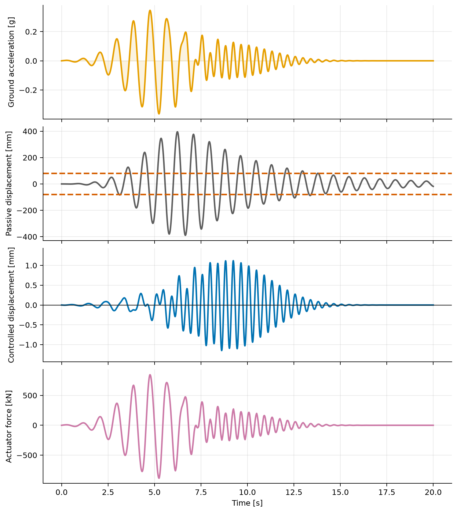
The passive comparison is not part of the constrained optimization and can exceed the \(80\) mm active-trajectory displacement limit.

Variables and units

Symbol	Meaning	Unit
\(t\)	Time	s
\(x\)	Relative or modal structural displacement	m
\(v\)	Relative or modal velocity	m/s
\(a_g\)	Prescribed ground acceleration	m/s²
\(u\)	Normalized actuator command	dimensionless
\(F\)	Ideal actuator force	N
\(m_s\)	Modal mass	kg
\(\omega_n\)	Undamped natural angular frequency	rad/s
\(\zeta\)	Modal damping ratio	dimensionless
\(J\)	Integral of normalized penalties	s

Modeling choices and limits

Relative/modal displacement is the correct coordinate for the base-excited SDOF equation; it should not be read as an absolute floor displacement or a multi-storey drift profile. A \(160\times4\) Lobatto mesh resolves both frequency components of the prescribed excitation.

The actuator is ideal: force follows \(u(t)\) instantaneously, with no force-rate limit, delay, saturation dynamics, stroke, power, energy, or attachment model. The controller has noncausal knowledge of the complete earthquake record. There is no state estimator, feedback law, robustness analysis, soil-structure interaction, higher mode, yielding, or uncertain parameter. These omissions make the example useful for an optimistic feedforward performance bound, not for controller deployment.

Run the example

python -m examples.structural_vibration_control

Save the figure without opening a window:

python -m examples.structural_vibration_control --save structural-vibration-control.png --no-show

Independent numerical validation

The collocation solution is reconstructed at 4,001 times. The force samples are linearly interpolated and the physical SDOF equations are independently integrated with a high-accuracy DOP853 solver. The same solver computes a passive response with \(u(t)=0\). The script compares the reintegrated state with the collocation state, checks the terminal rest condition and all dense bounds, and integrates squared physical force.

Quantity	Verified value
Objective \(J\)	\(0.02300351\)
Passive peak relative/modal displacement	\(395.2115\ \mathrm{mm}\)
Controlled peak relative/modal displacement	\(1.1492\ \mathrm{mm}\)
Peak ideal actuator force	\(885.675\ \mathrm{kN}\)
Integral squared actuator force	\(1.127056\times10^{12}\ \mathrm{N^2\,s}\)
Maximum forward displacement error	\(4.844\times10^{-5}\ \mathrm m\)
Maximum forward velocity error	\(6.712\times10^{-4}\ \mathrm{m/s}\)
Maximum dense path-bound violation	\(0\) at printed precision

The dramatic reduction from \(395.2115\) mm to \(1.1492\) mm is possible partly because the optimizer sees the entire future excitation and commands an ideal actuator. It is a numerical result for this deterministic teaching model, not an expected reduction for a causal real-world controller.

Source code

See the complete runnable example: examples/structural_vibration_control.py.