Finite-Horizon Linear-Quadratic Regulator

Background

A linear-quadratic regulator (LQR) balances state regulation against control effort. It is one of the few optimal-control problems with a complete continuous-time reference solution, so it is useful for checking a numerical transcription rather than merely demonstrating that an optimizer terminates.

This scalar problem includes a running cost, a free terminal state, and a terminal penalty. Pockit's collocation result is compared point by point with an independently integrated Riccati solution.

Problem formulation

For the linear dynamics

\[ \dot x=Ax+Bu,\qquad x(0)=x_0, \]

minimize

\[ J=\int_0^T\left(Qx^2+Ru^2\right)\,\mathrm{d}t +\frac{F}{2}x(T)^2. \]

The numerical values are

\[ A=-1,\quad B=1,\quad Q=1,\quad R=0.1, \quad F=1,\quad x_0=1,\quad T=1. \]

The terminal state \(x(T)\) is free. There are no state or control bounds; the positive weights \(Q\), \(R\), and \(F\) make the scalar problem strictly convex in the control.

Riccati reference solution

Write the optimal value function as

\[ V(t,x)=\frac{1}{2}P(t)x^2. \]

Minimizing the Hamilton-Jacobi-Bellman equation with respect to \(u\) gives

\[ u^*(t)=-\frac{B P(t)}{2R}x^*(t). \]

The scalar Riccati equation and terminal condition are

\[ \dot P=-2Q-2AP+\frac{B^2P^2}{2R}, \qquad P(T)=F. \]

After integrating \(P\) backward, the reference state is obtained from

\[ \dot x^*=\left(A-\frac{B^2P}{2R}\right)x^*, \qquad x^*(0)=x_0, \]

and the exact optimal value for this initial condition is

\[ J^*=\frac{1}{2}P(0)x_0^2. \]

The example computes this reference with high-accuracy solve_ivp calls that are independent of Pockit's collocation equations and Ipopt.

Variables and units

This benchmark is nondimensional.

Symbol	Meaning	Value or unit
\(t\)	Normalized time	-
\(x\)	Scalar regulation error	-
\(u\)	Scalar control	-
\(A,B\)	Dynamics coefficients	\(-1,1\)
\(Q,R\)	Running state and control weights	\(1,0.1\)
\(F\)	Terminal-state weight	\(1\)

Modeling choices and limitations

The implementation uses one Lobatto phase on \([0,1]\), with eight mesh intervals and six points per interval. A system-level variable named x_final represents the free terminal state and is tied to the phase endpoint; this permits a terminal penalty without fixing the endpoint value.

The model is intentionally scalar, linear, unconstrained, and nondimensional. It validates objective construction, a free terminal state, and trajectory accuracy. Constrained, nonlinear, stochastic, or estimator-coupled control requires a richer formulation and generally loses this closed-form reference.

Run the example

python -m examples.linear_quadratic_regulator

Save the figure without opening a window:

python -m examples.linear_quadratic_regulator --save lqr.png --no-show

The example follows the common pipeline:

system, phase = build_problem()
guess = initial_guess(phase)
solution = solve_problem(system, guess)
plot_solution(solution)

Verified result

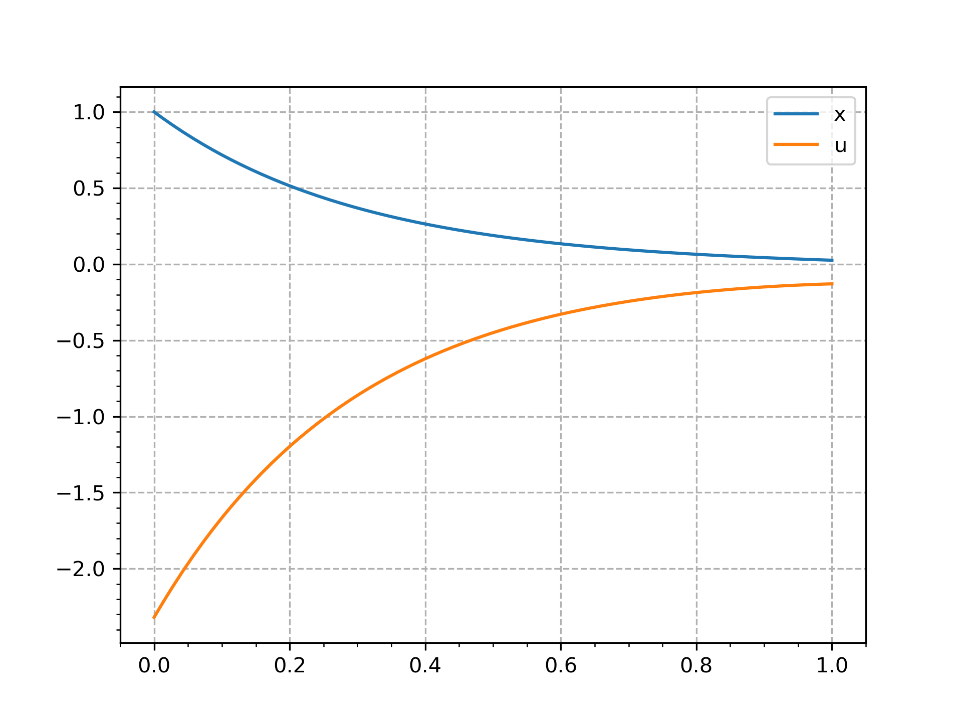
The script reconstructs the collocation state and control at 2,001 times and compares them with the independently integrated Riccati reference.

Quantity	Verified value
Objective \(J\)	\(0.231913974452\)
Terminal state \(x(1)\)	\(0.025836906771\)
Maximum state error against Riccati solution	\(6.104\times10^{-9}\)
Maximum control error against Riccati solution	\(1.303\times10^{-6}\)
Objective error against \(\tfrac12P(0)x_0^2\)	\(4.149\times10^{-14}\)

The terminal state is small but not fixed to zero: its optimized value reflects the stated trade-off between residual error and control effort. The numerical objective agrees with the continuous Riccati value to nearly machine precision.

Source code

See the complete runnable example: examples/linear_quadratic_regulator.py.