Minimum-Wind-Stress Ocean Inertial Current

Background

Wind transfers horizontal momentum into the ocean surface. After a wind event, an approximately homogeneous upper-ocean layer can rotate near the local inertial frequency because of the Coriolis force. This response is often studied first with a one-layer, or slab-ocean, model before adding vertical structure and turbulent mixing.

This example asks an inverse forcing question. A 50 m mixed layer at \(45^\circ\) N starts at rest. What spatially uniform, two-component surface stress history drives the mixed layer to an eastward current of \(0.20\ \mathrm{m/s}\) after 24 hours while minimizing squared stress? Treating the complete stress history as a decision variable creates a compact optimal-control benchmark with a closed-form solution.

The optimized stress is an idealized scientific forcing experiment. It is not a claim that real winds can be commanded or forecast exactly.

Slab-ocean model

Let \(u\) and \(v\) denote eastward and northward mixed-layer current, and let \(\tau_x\) and \(\tau_y\) be the corresponding surface-stress components. With time measured in hours, the damped \(f\)-plane momentum equations are

\[ \begin{aligned} \dot u &= f v-r u+b\tau_x,\\ \dot v &=-f u-r v+b\tau_y, \end{aligned} \qquad b=\frac{3600}{\rho H}. \]

Here \(f=2\Omega\sin\phi\) is converted from \(\mathrm{s^{-1}}\) to \(\mathrm{h^{-1}}\), \(r\) is a linear Rayleigh-damping rate, \(\rho\) is seawater density, and \(H\) is mixed-layer depth. The signs correspond to east-north coordinates in the Northern Hemisphere: an unforced current rotates clockwise.

The numerical values are

\[ \begin{gathered} \phi=45^\circ,\qquad \Omega=7.2921159\times10^{-5}\ \mathrm{rad/s},\\ f=0.3712539314\ \mathrm{h^{-1}},\qquad \frac{2\pi}{f}=16.9242\ \mathrm h,\\ \rho=1025\ \mathrm{kg/m^3},\qquad H=50\ \mathrm m,\qquad r=(48\ \mathrm h)^{-1},\\ b=0.07024390244\, \frac{\mathrm{m/s}}{\mathrm h\,(\mathrm{N/m^2})}. \end{gathered} \]

Objective, endpoints, and path bounds

The fixed horizon is \(T=24\ \mathrm h\). The normalized mean forcing effort is

\[ \min_{\tau_x,\tau_y} J =\frac{1}{T}\int_0^T \left[ \left(\frac{\tau_x}{\tau_s}\right)^2 +\left(\frac{\tau_y}{\tau_s}\right)^2 \right]\,\mathrm dt, \qquad \tau_s=0.25\ \mathrm{N/m^2}. \]

The scale \(\tau_s\) makes \(J\) dimensionless and does not change the minimizing stress history. The endpoint conditions are

\[ \begin{bmatrix}u(0)\\v(0)\end{bmatrix} =\begin{bmatrix}0\\0\end{bmatrix}\ \mathrm{m/s}, \qquad \begin{bmatrix}u(T)\\v(T)\end{bmatrix} =\begin{bmatrix}0.20\\0\end{bmatrix}\ \mathrm{m/s}. \]

Component-wise path bounds keep the transcription in a stated physical range:

\[ |u(t)|,|v(t)|\le0.35\ \mathrm{m/s}, \qquad |\tau_x(t)|,|\tau_y(t)|\le0.30\ \mathrm{N/m^2}. \]

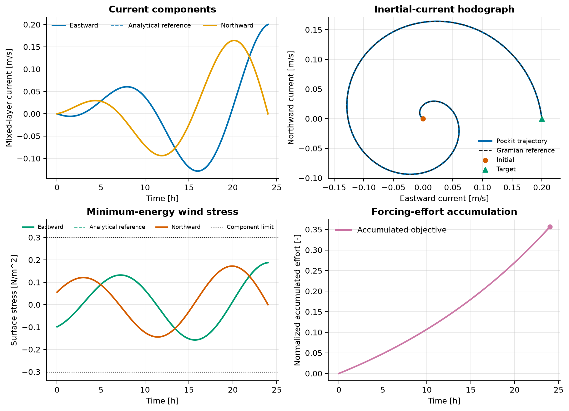
These are component limits, not Euclidean-magnitude limits. The exact unconstrained optimum stays strictly inside every bound, so it is also the solution of this constrained problem.

Exact Gramian solution

Write \(\mathbf{x}=[u,v]^\mathsf{T}\) and \(\boldsymbol{\tau}=[\tau_x,\tau_y]^\mathsf{T}\). Then

\[ \dot{\mathbf{x}}=A\mathbf{x}+B\boldsymbol{\tau}, \qquad A=\begin{bmatrix}-r&f\\-f&-r\end{bmatrix}, \qquad B=bI_2. \]

The state-transition matrix is

\[ \Phi(t)=e^{At} =e^{-rt} \begin{bmatrix} \cos(ft)&\sin(ft)\\ -\sin(ft)&\cos(ft) \end{bmatrix}. \]

Because damping and forcing are isotropic, the finite-horizon controllability Gramian reduces to a scalar times the identity:

\[ W(T)=\int_0^T \Phi(T-s)BB^\mathsf{T}\Phi(T-s)^\mathsf{T}\,\mathrm ds =wI_2, \qquad w=b^2\frac{1-e^{-2rT}}{2r}. \]

For \(\mathbf{x}(0)=0\) and fixed target \(\mathbf{x}_T\), the unique minimum-energy stress is

\[ \boldsymbol{\tau}^*(t) =B^\mathsf{T}\Phi(T-t)^\mathsf{T}W(T)^{-1}\mathbf{x}_T, \]

and its unnormalized energy is

\[ E^*=\int_0^T \boldsymbol{\tau}^{*\mathsf{T}}\boldsymbol{\tau}^*\,\mathrm dt =\mathbf{x}_T^\mathsf{T}W(T)^{-1}\mathbf{x}_T. \]

The corresponding current has the closed form

\[ \mathbf{x}^*(t)= \frac{b^2e^{-r(T-t)}(1-e^{-2rt})}{2rw} \begin{bmatrix} \cos(f(T-t))&-\sin(f(T-t))\\ \sin(f(T-t))&\cos(f(T-t)) \end{bmatrix} \mathbf{x}_T. \]

This analytical pair supplies a feasible initial guess and, more importantly, an external reference for the numerical optimum.

Variables and units

Symbol	Meaning	Unit
\(t,T\)	Time and forcing horizon	h
\(u,v\)	Eastward and northward mixed-layer current	m/s
\(\tau_x,\tau_y\)	Eastward and northward surface stress	N/m²
\(\tau_s\)	Objective normalization scale	N/m²
\(f\)	Coriolis parameter in the hourly time coordinate	h⁻¹
\(r\)	Linear momentum-damping rate	h⁻¹
\(\rho\)	Seawater density	kg/m³
\(H\)	Mixed-layer depth	m
\(b\)	Stress-to-current tendency gain	\((\mathrm{m/s})/[\mathrm h(\mathrm{N/m^2})]\)

Discretization and independent checks

The default solve uses 48 uniform Lobatto mesh intervals with four points per interval. The script reconstructs the solution at 4,001 times and performs four checks outside the nonlinear-program convergence test:

1. It compares current and stress point by point with the Gramian solution.
2. It linearly interpolates the optimized stress and reintegrates both physical momentum equations with an independent high-accuracy DOP853 solver.
3. It compares the collocation objective and dense trapezoidal stress energy with the exact minimum energy.
4. It checks endpoint residuals and every component bound on the dense grid.

The --quick mode uses 32 intervals with the same four-point polynomial order. It remains an analytical smoke test rather than merely checking solver status.

Verified result

Quantity	Default-mesh value
Normalized objective \(J\)	\(0.3562380575\)
Exact normalized objective	\(0.3562380568\)
Stress energy \(E\)	\(0.5343570891\ (\mathrm{N/m^2})^2\,\mathrm h\)
Peak current speed	\(0.20000000\ \mathrm{m/s}\)
Peak stress magnitude	\(0.18767921\ \mathrm{N/m^2}\)
Maximum current error against the exact solution	\(1.279\times10^{-7}\ \mathrm{m/s}\)
Maximum stress error against the exact solution	\(9.652\times10^{-6}\ \mathrm{N/m^2}\)
Maximum independent forward-integration error	\(1.705\times10^{-7}\ \mathrm{m/s}\)
Maximum dense path-bound violation	\(0\)

The current hodograph makes the Coriolis rotation visible. The optimized stress also rotates, while its envelope increases toward the terminal time because the response to later forcing is attenuated less before reaching the target.

Modeling scope and limits

The slab model assumes a horizontally uniform and vertically homogeneous layer with constant depth, density, Coriolis parameter, and linear drag. It omits pressure-gradient forcing, nonlinear advection, stratification, entrainment, turbulent vertical structure, coastlines, bathymetry, waves, and air-sea feedback. Rayleigh drag is a reduced dissipation model, not a turbulence closure.

The calculation also assumes that the entire deterministic stress history is available to the optimizer. Real ocean prediction would require atmospheric forcing uncertainty, data assimilation, and usually feedback or receding- horizon estimation. Use this example to verify optimal-control transcription and reason about rotating linear dynamics, not as an operational wind or ocean forecast.

Run the example

Run the verified default mesh:

python -m examples.ocean_inertial_current

Run a faster analytical smoke test:

python -m examples.ocean_inertial_current --quick --no-show

Save the figure without opening a window:

python -m examples.ocean_inertial_current --save ocean-inertial-current.png --no-show

Source code

See the complete runnable example: examples/ocean_inertial_current.py.