Ramsey Growth Model

Background

The Ramsey growth model asks how a social planner should divide output between current consumption and investment. Consuming more raises utility today; investing more builds capital and expands future output. This example computes a 30-year transition from a capital-poor economy to its modified-golden-rule steady state.

The variables are normalized per worker. The model is deterministic and is intended to demonstrate optimal control in macroeconomics, not to forecast a particular economy.

Problem formulation

Production per worker follows a Cobb-Douglas technology

\[ y(t)=A k(t)^\alpha, \]

where \(k(t)\) is capital and \(c(t)\) is consumption, both per worker. Capital accumulation obeys the resource balance

\[ \dot k=A k^\alpha-\delta k-c. \]

The planner maximizes discounted logarithmic utility over a fixed horizon \(T=30\) years:

\[ \max_{k,c}\ W=\int_0^T e^{-\rho t}\log c(t)\,\mathrm dt. \]

Pockit minimizes \(-W\). With productivity \(A=1\), capital share \(\alpha=0.33\), depreciation \(\delta=0.06\ \mathrm{year^{-1}}\), and discount rate \(\rho=0.04\ \mathrm{year^{-1}}\), the modified-golden-rule steady state satisfies

\[ \alpha A(k^*)^{\alpha-1}=\rho+\delta, \qquad k^*=\left(\frac{\alpha A}{\rho+\delta}\right)^{\!1/(1-\alpha)}, \]

and steady consumption is

\[ c^*=A(k^*)^\alpha-\delta k^*. \]

The economy starts below the steady state and must reach it at the horizon:

\[ k(0)=0.55k^*, \qquad k(T)=k^*. \]

The path bounds keep the logarithm defined and the numerical search in an economically meaningful region:

\[ 0.20k^*\le k(t)\le1.20k^*, \qquad 0.05c^*\le c(t)\le1.80c^*. \]

Parameters, variables, and units

Symbol	Meaning	Value or unit
\(t\)	Time	years
\(k\)	Capital per worker	normalized capital/worker
\(c\)	Consumption per worker	normalized flow/worker/year
\(y\)	Output per worker	normalized flow/worker/year
\(A\)	Productivity	\(1.0\)
\(\alpha\)	Capital share	\(0.33\)
\(\delta\)	Depreciation rate	\(0.06\ \mathrm{year^{-1}}\)
\(\rho\)	Utility discount rate	\(0.04\ \mathrm{year^{-1}}\)
\(k^*\)	Modified-golden-rule capital	\(5.941573\)
\(c^*\)	Steady-state consumption	\(1.443982\)

Analytical validation

On an interior arc, the current-value first-order conditions give the Ramsey Euler equation

\[ \frac{\dot c}{c} =\alpha A k^{\alpha-1}-\delta-\rho. \]

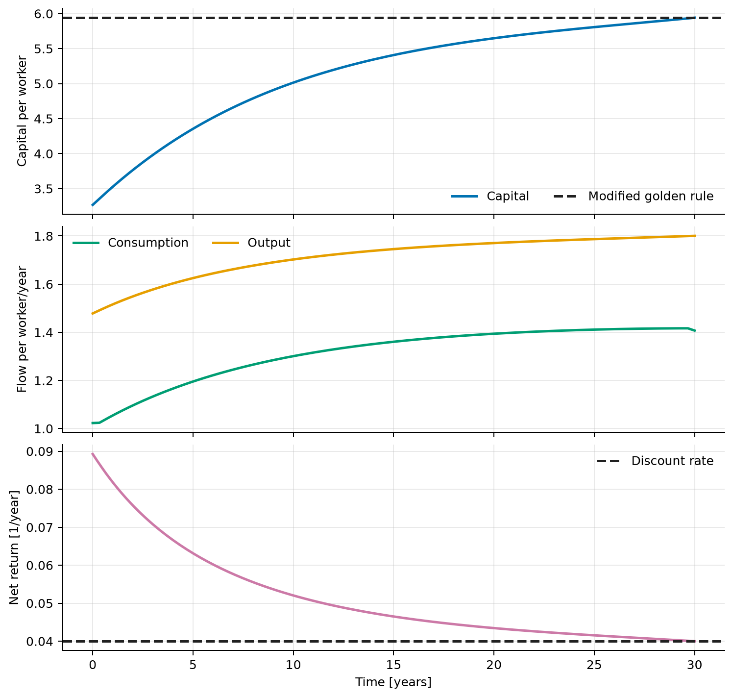
The right-hand side is the net marginal return on capital minus impatience. It approaches zero as the trajectory reaches \(k^*\). The script evaluates this equation independently at control-grid midpoints, excluding the first and last year where the fixed endpoint has the strongest numerical influence.

Modeling choices

The fixed terminal capital turns the infinite-horizon steady-state idea into a well-posed finite-horizon transition. Terminal consumption is free and there is no terminal utility term. Explicit positive consumption bounds protect the logarithm; the reported solution remains on an interior consumption arc.

The implementation uses a \(90\times2\) Lobatto mesh, corresponding to piecewise-linear capital and consumption histories over four-month intervals. The initial guess approximately satisfies the resource balance while moving capital linearly toward \(k^*\).

Run the example

python -m examples.ramsey_growth

Save the figure without opening a window:

python -m examples.ramsey_growth --save ramsey-growth.png --no-show

system, phase = build_problem()
guess = initial_guess(phase)
solution = solve_problem(system, guess)
plot_solution(solution)

Verified result

The state and control are reconstructed at 4,001 times and checked against all path and terminal constraints. The independently evaluated interior Euler residual provides an economic optimality diagnostic in addition to NLP solver convergence.

Quantity	Verified value
Discounted welfare \(W\)	\(4.22687109\)
Steady-state capital \(k^*\)	\(5.941573\)
Steady-state consumption \(c^*\)	\(1.443982\)
Interior Euler-equation RMS residual	\(8.024\times10^{-6}\ \mathrm{year^{-1}}\)
Maximum dense path-bound violation	\(0\)

Capital rises monotonically toward the imposed steady state. Consumption also rises, while the net marginal return converges toward the discount rate as predicted by the modified golden rule.

Source code

See the complete runnable example: examples/ramsey_growth.py.