Humanoid Operational-Space and Whole-Body Control

Background

Operational-space control (OSC) describes a robot task in Cartesian space, while whole-body control (WBC) uses redundant joint motion to satisfy lower priority goals without disturbing the primary task. This example gives a small, inspectable version of that hierarchy: a planar humanoid upper body tracks a moving right-hand target while the left hand approaches a separate target and the torso returns upright.

This is deliberately a teaching example at the acceleration level. It uses identity joint-space acceleration dynamics in a stabilized shoulder frame. It is not a production floating-base/contact-force WBC model: it does not include a rigid-body mass matrix, gravity compensation, torque limits, contacts, friction cones, center-of-pressure constraints, or balance.

Kinematic model

The five joint coordinates are

\[ \boldsymbol q= \begin{bmatrix} q_T&q_{RS}&q_{RE}&q_{LS}&q_{LE} \end{bmatrix}^{\mathsf T}, \]

representing torso posture, right shoulder and elbow, and left shoulder and elbow. The shoulder origin is fixed at \(\boldsymbol s=[0,L_T]^{\mathsf T}\), with

\[ L_T=0.60\ \mathrm m,\qquad L_1=0.38\ \mathrm m,\qquad L_2=0.30\ \mathrm m. \]

The right- and left-hand positions are

\[ \boldsymbol p_R(\boldsymbol q) =\boldsymbol s+ \begin{bmatrix} L_1\cos q_{RS}+L_2\cos(q_{RS}+q_{RE})\\ L_1\sin q_{RS}+L_2\sin(q_{RS}+q_{RE}) \end{bmatrix}, \]

\[ \boldsymbol p_L(\boldsymbol q) =\boldsymbol s+ \begin{bmatrix} -L_1\cos q_{LS}-L_2\cos(q_{LS}+q_{LE})\\ L_1\sin q_{LS}+L_2\sin(q_{LS}+q_{LE}) \end{bmatrix}. \]

Because the hand tasks are expressed in the stabilized shoulder frame, \(q_T\) does not enter either hand kinematics. This deliberate simplification makes the null-space structure visible.

Primary right-hand task

The fixed horizon is \(T=2.5\ \mathrm s\). Define

\[ \tau=\frac{t}{T}, \qquad h(\tau)=10\tau^3-15\tau^4+6\tau^5, \]

\[ \dot h =\frac{30\tau^2-60\tau^3+30\tau^4}{T}, \qquad \ddot h =\frac{60\tau-180\tau^2+120\tau^3}{T^2}. \]

Starting from

\[ \boldsymbol q(0) = \begin{bmatrix} 0.25&-0.45&0.95&0.60&-1.10 \end{bmatrix}^{\mathsf T}, \qquad \dot{\boldsymbol q}(0)=\boldsymbol 0, \]

the desired right-hand trajectory is

\[ \boldsymbol p_{R,d}(t) =\boldsymbol p_R(\boldsymbol q(0)) + \begin{bmatrix} 0.04\\0.08 \end{bmatrix} h(\tau). \]

Numerically, the hand moves from approximately \([0.605445,0.578541]^{\mathsf T}\ \mathrm m\) to \([0.645445,0.658541]^{\mathsf T}\ \mathrm m\). Its desired velocity and acceleration use \(\dot h\) and \(\ddot h\).

Let

\[ J=\frac{\partial\boldsymbol p_R}{\partial\boldsymbol q}, \qquad \dot J=\sum_{i=1}^{5}\frac{\partial J}{\partial q_i}\dot q_i. \]

The feedback acceleration reference is

\[ \boldsymbol a_{\mathrm{ref}} =\ddot{\boldsymbol p}_{R,d} +36\left(\boldsymbol p_{R,d}-\boldsymbol p_R\right) +12\left(\dot{\boldsymbol p}_{R,d}-J\dot{\boldsymbol q}\right). \]

The exact task hierarchy used by the state dynamics is

\[ J^\#=J^{\mathsf T}\left(JJ^{\mathsf T}\right)^{-1}, \qquad N=I-J^\#J, \]

\[ \ddot{\boldsymbol q} =J^\#\left(\boldsymbol a_{\mathrm{ref}}-\dot J\dot{\boldsymbol q}\right) +N\boldsymbol z. \]

The Pockit state is \(\boldsymbol x=[\boldsymbol q^{\mathsf T}, \dot{\boldsymbol q}^{\mathsf T}]^{\mathsf T}\), the control is the five-dimensional null-space command \(\boldsymbol z\), and

\[ \dot{\boldsymbol x} = \begin{bmatrix} \dot{\boldsymbol q}\\ \ddot{\boldsymbol q} \end{bmatrix}. \]

For this model, the right-hand Jacobian only uses \(q_{RS}\) and \(q_{RE}\). Its analytical pseudoinverse therefore gives

\[ N=\operatorname{diag}(1,0,0,1,1), \]

so torso and left-arm accelerations cannot alter the primary right-hand acceleration.

Null-space objective and constraints

The left-hand target is generated by \((q_{LS},q_{LE})=(-0.45,1.00)\), giving

\[ \boldsymbol p_L^\star \approx \begin{bmatrix} -0.597927&0.591519 \end{bmatrix}^{\mathsf T}\ \mathrm m. \]

With \(J_L=\partial\boldsymbol p_L/\partial\boldsymbol q\), the secondary objective is

\[ \begin{aligned} \min_{\boldsymbol z}\quad \int_0^T &120\lVert\boldsymbol p_L-\boldsymbol p_L^\star\rVert_2^2 +3\lVert J_L\dot{\boldsymbol q}\rVert_2^2\\ &+20q_T^2 +0.03\lVert\dot{\boldsymbol q}\rVert_2^2 +0.01\lVert\boldsymbol z\rVert_2^2 \,\mathrm dt. \end{aligned} \]

The joint ranges are

\[ \begin{aligned} -0.55&\le q_T\le0.55,& -1.8&\le q_{RS}\le1.2,\\ 0.35&\le q_{RE}\le1.8,& -2.2&\le q_{LS},q_{LE}\le2.2. \end{aligned} \]

All joint speeds satisfy \(|\dot q_i|\le3\ \mathrm{rad/s}\), and all null-space commands satisfy \(|z_i|\le10\ \mathrm{rad/s^2}\). The positive right-elbow lower bound keeps the \(2\times2\) arm Jacobian away from its straight-arm singularity. The terminal joint state is free.

Variables and units

Symbol	Meaning	Unit
\(q_T\)	Torso posture angle	rad
\(q_{RS},q_{RE}\)	Right shoulder and elbow angles	rad
\(q_{LS},q_{LE}\)	Left shoulder and elbow angles	rad
\(\dot{\boldsymbol q}\)	Joint velocities	rad/s
\(\boldsymbol z\)	Null-space joint-acceleration command	rad/s²
\(\boldsymbol p_R,\boldsymbol p_L\)	Hand positions	m
\(J,J_L\)	Hand Jacobians	m/rad

Modeling choices

Planar revolute coordinates avoid the redundant quaternion and unit-norm constraint that a spatial attitude model would require. The stabilized shoulder frame and identity acceleration dynamics isolate the task-priority idea from rigid-body dynamics. The script evaluates the closed form of \(J^\#=J^{\mathsf T}(JJ^{\mathsf T})^{-1}\); this is mathematically identical to the matrix expression but substantially reduces symbolic Hessian generation time.

The problem uses one fixed-time Lobatto phase with 10 mesh intervals and four points per interval. A quintic joint-space initial guess moves toward the secondary targets with zero endpoint velocity. After optimization, all states and controls are reconstructed at 4,001 uniformly spaced physical times. The script checks every joint-angle, joint-speed, and null-acceleration bound on that dense grid in addition to evaluating the task hierarchy.

Run the example

From the repository root, run:

python -m examples.humanoid_whole_body_control

Symbolic differentiation for this nonlinear hierarchy makes the first run slower than the other introductory examples. To save the figure without opening an interactive window:

python -m examples.humanoid_whole_body_control --save humanoid-whole-body-control.png --no-show

Key implementation

joint_angles = sp.Matrix(phase.x[:5])
joint_velocities = sp.Matrix(phase.x[5:])
z = sp.Matrix(phase.u)

right_hand, left_hand = _symbolic_hand_positions(joint_angles)
J = right_hand.jacobian(joint_angles)
J_left = left_hand.jacobian(joint_angles)
J_dot = sp.zeros(2, 5)
for i in range(5):
    J_dot += J.diff(joint_angles[i]) * joint_velocities[i]

# Closed form of J.T * (J * J.T)^-1 for the nonsingular right 2R arm.
J_arm = J[:, 1:3]
det_J_arm = (
    J_arm[0, 0] * J_arm[1, 1] - J_arm[0, 1] * J_arm[1, 0]
)
J_arm_inverse = sp.Matrix(
    [[J_arm[1, 1], -J_arm[0, 1]],
     [-J_arm[1, 0], J_arm[0, 0]]]
) / det_J_arm
J_pinv = sp.zeros(5, 2)
J_pinv[1:3, :] = J_arm_inverse
N = sp.diag(1.0, 0.0, 0.0, 1.0, 1.0)

a_ref = (
    desired_acceleration
    + 36.0 * (desired_position - right_hand)
    + 12.0 * (desired_velocity - J * joint_velocities)
)
qdd = J_pinv * (a_ref - J_dot * joint_velocities) + N * z
phase.set_dynamics([*joint_velocities, *qdd])

The full source also defines the secondary integral cost, joint bounds, dynamics-informed initial guess, dense numerical hierarchy and bound checks, and all plots.

Verified result

The script verifies the hierarchy numerically after every successful solve:

Check	Verified value
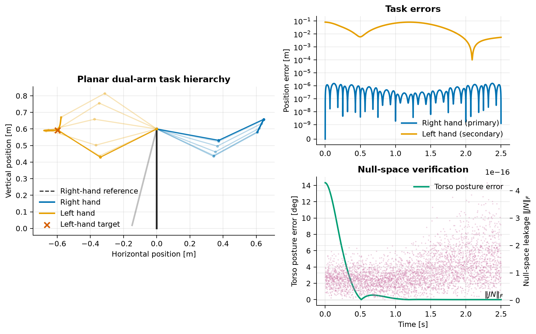
Maximum null-space leakage \(\max_t\lVert JN\rVert_F\)	\(4.286\times10^{-16}\)
Maximum right-hand tracking error	\(1.535\times10^{-6}\ \mathrm m\)
Initial left-hand target error	\(0.0820\ \mathrm m\)
Final left-hand target error	\(0.0055\ \mathrm m\)
Maximum dense path-bound violation	\(0\)

Thus the lower-priority motion improves the left-hand task by more than an order of magnitude while preserving the right-hand trajectory to numerical precision. The figure shows sampled arm poses, both hand trajectories, task errors, torso regulation, and the measured null-space leakage from the dense history without clipping the plotted diagnostic values.

Source code

See the complete runnable example: examples/humanoid_whole_body_control.py.