Multi-Phase Electric-Vehicle Eco-Driving

Background

An energy-aware vehicle should adapt its speed to road conditions rather than follow one profile everywhere. This example joins a one-kilometer urban segment to a two-kilometer arterial segment. The segments have different speed limits and grade-resistance terms, while the crossing time and crossing speed are free. The vehicle must stop at both ends and trades accumulated energy against trip time.

Separate phases make the road transition explicit and provide a reusable pattern for route segments, speed zones, charging stops, or other discrete operating regimes.

Problem formulation

For segment \(j\in\{u,a\}\), the state is distance, speed, and an accumulated energy proxy, \(x_j=(d_j,v_j,E_j)\). The control \(a_j\) is a bounded acceleration command. The dynamics are

\[ \begin{aligned} \dot d_j &= v_j, \\ \dot v_j &= a_j-0.06v_j^2-g_j, \\ \dot E_j &= 0.08v_j+0.04v_j^3+0.03a_j^2, \end{aligned} \]

where \(g_u=0.025\) for the uphill urban segment and \(g_a=-0.010\) for the downhill arterial segment. Distances and endpoint conditions are

\[ \begin{aligned} (d_u(0),v_u(0),E_u(0))&=(0,0,0), \\ d_u(t_s)&=1, \\ d_a(t_s)&=1, \\ (d_a(t_f),v_a(t_f))&=(3,0). \end{aligned} \]

Speed and energy are continuous at the road transition:

\[ v_u(t_s)=v_a(t_s)=v_s, \qquad E_u(t_s)=E_a(t_s)=E_s. \]

The path bounds are

\[ \begin{aligned} 0\le v_u&\le0.60, & -1.20\le a_u&\le1.00, \\ 0\le v_a&\le1.50, & -1.20\le a_a&\le1.00, \end{aligned} \]

with speed in kilometers per minute. Thus, the two speed limits are 36 and 90 kilometers per hour. The event and horizon bounds are

\[ 1.70\le t_s\le5.00, \quad 1.50\le t_f-t_s\le5.00, \quad 3.20\le t_f\le9.00. \]

The objective is

\[ \min J=E_a(t_f)+0.15t_f. \]

Variables and units

Symbol	Meaning	Unit
\(t\)	Time	min
\(d\)	Distance along the route	km
\(v\)	Vehicle speed	km/min
\(a\)	Acceleration command	km/min\(^2\)
\(E\)	Accumulated energy proxy	normalized
\(g_j\)	Grade-resistance acceleration term	km/min\(^2\)
\(t_s,t_f\)	Road-transition and final times	min

Modeling choices

The urban and arterial roads are two Lobatto phases, each with 40 mesh intervals and two interpolation points per interval. The resulting piecewise-linear speed and acceleration profiles preserve their nodal bounds throughout every interval. Shared static parameters connect speed, accumulated energy, and time across the event. Position is fixed to the known segment boundary on each side, so no extra position parameter is required. The implementation also checks both phases at 2,001 uniformly spaced times after the solve.

The energy state integrates rolling, aerodynamic, and command-effort terms. It is a transparent normalized proxy rather than a detailed battery model. Static bounds keep event times and energy guesses physically scaled during nonlinear optimization.

Run the example

python -m examples.multiphase_electric_vehicle

Save the figure without opening a window:

python -m examples.multiphase_electric_vehicle --save electric-vehicle.png --no-show

Key implementation

urban = system.new_phase(
    ["position_u", "speed_u", "energy_u"], ["acceleration_u"]
)
arterial = system.new_phase(
    ["position_a", "speed_a", "energy_a"], ["acceleration_a"]
)

_configure_segment(
    urban, grade=0.025, speed_limit=URBAN_SPEED_LIMIT,
    boundaries=([0.0, 0.0, 0.0], [DISTANCE_SWITCH, v_s, e_s]),
    times=(0.0, t_s),
)
_configure_segment(
    arterial, grade=-0.010, speed_limit=ARTERIAL_SPEED_LIMIT,
    boundaries=([DISTANCE_SWITCH, v_s, e_s],
                [DISTANCE_FINAL, 0.0, e_f]),
    times=(t_s, t_f),
)
system.set_phase([urban, arterial])
system.set_objective(e_f + 0.15 * t_f)

Verified result

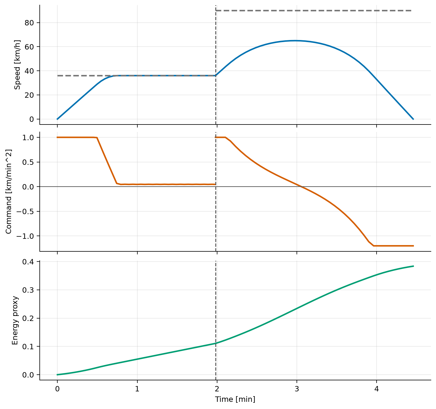
Ipopt terminates successfully with objective \(1.05215819\). The vehicle reaches the road transition at \(t_s=1.980266\ \mathrm{min}\) and exactly the urban speed limit, \(36.000\ \mathrm{km/h}\). It completes the three-kilometer trip in \(t_f=4.456853\ \mathrm{min}\). The arterial speed peaks at \(65.001\ \mathrm{km/h}\), below its \(90\ \mathrm{km/h}\) limit. The speed mismatch across the phase boundary is below \(2\times10^{-6}\), and the dense speed and acceleration checks show no path-bound violation at the reported precision.

Source code

See the complete runnable example: examples/multiphase_electric_vehicle.py.