Minimum-Fuel Planar Free-Flying Robot

Background

A free-flying inspection robot or spacecraft must translate and rotate without support from the environment. In this planar example, two actuator modules produce force along the body axis. Each module contains opposed one-sided jets, so it can generate force in either body-axis direction, while the difference between the two module forces generates a yaw moment.

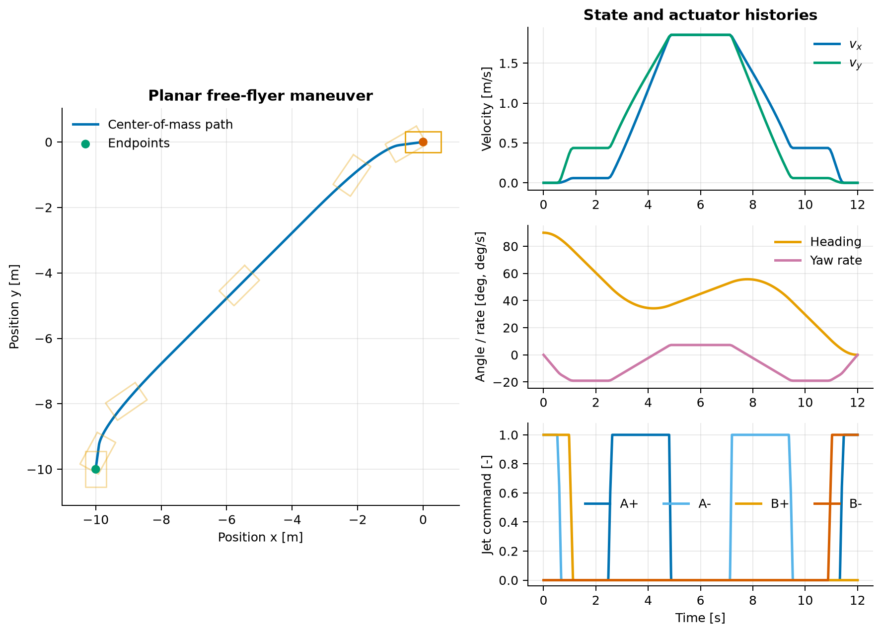
The robot must move from \((-10,-10)\) to the origin, stop, and change its heading from \(90^\circ\) to zero in 12 seconds. The optimization minimizes a normalized propellant-use proxy.

Problem formulation

The state and actuator vectors are

\[ \boldsymbol{x} = \begin{bmatrix} x&y&v_x&v_y&\theta&\omega \end{bmatrix}^{\mathsf T}, \]

\[ \boldsymbol{u} = \begin{bmatrix} u_{A+}&u_{A-}&u_{B+}&u_{B-} \end{bmatrix}^{\mathsf T}. \]

The signed module thrusts are formed from antagonistic jets:

\[ T_A=u_{A+}-u_{A-}, \qquad T_B=u_{B+}-u_{B-}. \]

With normalized translational mass and yaw inertia, and moment coefficients \(\alpha=\beta=0.2\), the dynamics are

\[ \begin{aligned} \dot x &= v_x, & \dot v_x &= (T_A+T_B)\cos\theta,\\ \dot y &= v_y, & \dot v_y &= (T_A+T_B)\sin\theta,\\ \dot\theta &= \omega, & \dot\omega &= \alpha T_A-\beta T_B. \end{aligned} \]

Every jet command is one-sided and bounded:

\[ 0\le u_{A+},u_{A-},u_{B+},u_{B-}\le1. \]

The objective is

\[ \min_{\boldsymbol{x},\boldsymbol{u}} \quad \int_0^{12} \left(u_{A+}+u_{A-}+u_{B+}+u_{B-}\right)\,\mathrm dt. \]

The fixed endpoint conditions are

\[ \boldsymbol{x}(0) = \begin{bmatrix} -10&-10&0&0&\pi/2&0 \end{bmatrix}^{\mathsf T}, \]

\[ \boldsymbol{x}(12) = \begin{bmatrix} 0&0&0&0&0&0 \end{bmatrix}^{\mathsf T}. \]

Variables and units

Lengths and time retain SI units. Forces, mass, yaw inertia, and propellant flow are normalized, so the actuator commands and objective are scaled.

Symbol	Meaning	Unit
\(t\)	Time	s
\(x,y\)	Center-of-mass position	m
\(v_x,v_y\)	Inertial velocity	m/s
\(\theta\)	Body heading	rad
\(\omega\)	Yaw rate	rad/s
\(u_{A+},u_{A-},u_{B+},u_{B-}\)	One-sided jet commands	-
\(T_A,T_B\)	Signed module thrusts	scaled
\(\alpha,\beta\)	Yaw-moment coefficients	scaled

Modeling choices

Attitude in a planar problem belongs to \(\mathrm{SO}(2)\), so one continuous heading angle is sufficient; a four-component quaternion and a unit-norm constraint would add redundant variables. The antagonistic-jet construction also matters for the objective: each physical jet command remains nonnegative, and firing either direction consumes propellant.

The example neglects external forces and uses normalized mass and inertia so that the guidance structure remains easy to inspect. It is a trajectory optimization model, not a high-fidelity spacecraft propulsion model.

The phase uses 160 Lobatto mesh intervals with two points per interval. This makes every jet command piecewise linear: endpoint bounds then hold throughout each interval, without the between-node overshoot possible with a high-order control polynomial. Ipopt's bound relaxation is disabled, and the returned commands are independently evaluated with V_u at 10,001 times.

The initial guess uses a quintic rest-to-rest profile for position and heading, then maps the approximate axial acceleration and yaw acceleration back to the four one-sided jets.

Run the example

From the repository root, run:

python -m examples.free_flying_robot

To save the plot without opening an interactive window:

python -m examples.free_flying_robot --save free-flying-robot.png --no-show

Key implementation

import numpy as np
import sympy as sp

from pockit.lobatto import System

system = System(0)
phase = system.new_phase(
    ["x", "y", "velocity_x", "velocity_y", "heading", "yaw_rate"],
    [
        "module_a_positive",
        "module_a_negative",
        "module_b_positive",
        "module_b_negative",
    ],
)
_, _, v_x, v_y, heading, yaw_rate = phase.x
u_ap, u_am, u_bp, u_bm = phase.u

thrust_a = u_ap - u_am
thrust_b = u_bp - u_bm
total_thrust = thrust_a + thrust_b
yaw_moment = 0.2 * thrust_a - 0.2 * thrust_b

phase.set_dynamics(
    [
        v_x,
        v_y,
        total_thrust * sp.cos(heading),
        total_thrust * sp.sin(heading),
        yaw_rate,
        yaw_moment,
    ]
)
phase.set_integral([sum(phase.u)])
phase.set_phase_constraint(list(phase.u), [0.0] * 4, [1.0] * 4, True)
phase.set_boundary_condition(
    [-10.0, -10.0, 0.0, 0.0, 0.5 * np.pi, 0.0],
    [0.0] * 6,
    0.0,
    12.0,
)
phase.set_discretization(160, 2)
system.set_phase([phase])
system.set_objective(phase.I[0])

The full script supplies the dynamics-informed initial guess, solves with bound_relax_factor=0.0, verifies the terminal state, rejects any solution whose 10,001-point V_u history leaves \([0,1]\), and draws the path together with sampled robot poses and actuator histories.

Verified result

The default solve terminates successfully with a normalized propellant proxy of

\[ J=7.915541559. \]

The 10,001-point interpolated command range is \([0.000000000,0.999999997]\), so all four jets remain within \([0,1]\) over the complete horizon, not only at collocation nodes. The numerical endpoint matches the requested zero position, velocity, heading, and yaw rate within the script's \(2\times10^{-7}\) absolute check.

Source code

See the complete runnable example: examples/free_flying_robot.py.