Almgren-Chriss Optimal Trade Execution

Background

Liquidating a large position creates a timing trade-off. Selling quickly reduces exposure to future price variation, but concentrated trading increases temporary market impact. The continuous-time Almgren-Chriss benchmark captures this trade-off with a quadratic cost and has a closed-form optimal schedule.

This example liquidates 100,000 shares during one trading day. Inventory, trading speed, and cost coefficients are normalized, so the objective is a dimensionless numerical benchmark rather than a currency estimate.

Problem formulation

Let \(x(t)\) be the fraction of the initial order still held and \(v(t)\) the sell rate in initial-inventory fractions per day. Inventory evolves as

\[ \dot x(t)=-v(t), \qquad 0\le t\le T=1. \]

Complete liquidation imposes

\[ x(0)=1, \qquad x(T)=0. \]

The normalized mean-variance objective is

\[ \min_{x,v}\;J=\int_0^T \left[\eta v(t)^2+\rho x(t)^2\right]\,\mathrm dt, \]

where \(\eta=0.05\) weights temporary market impact and \(\rho=0.20\) weights inventory risk. The path constraints are

\[ 0\le x(t)\le1, \qquad 0\le v(t)\le3. \]

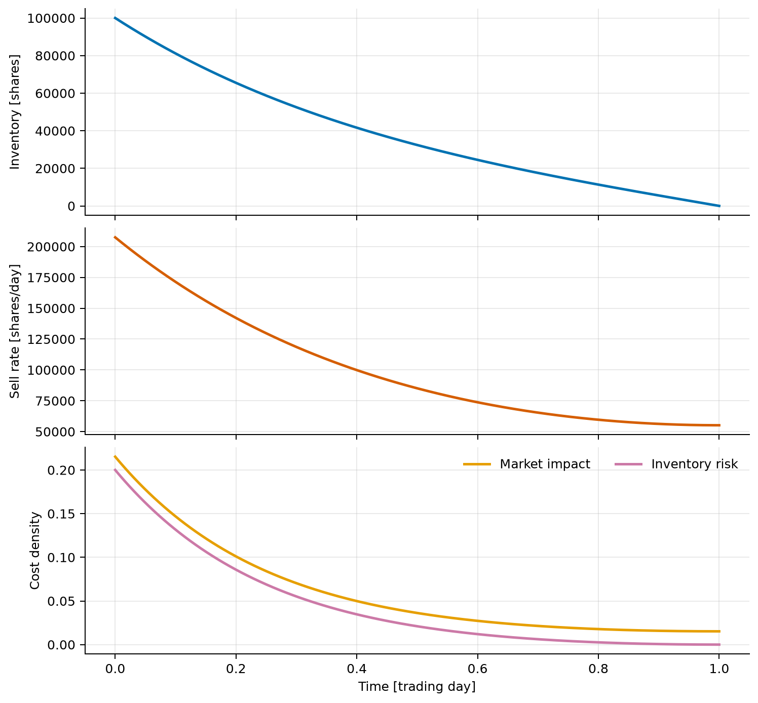
For an order of \(Q=100{,}000\) shares, physical inventory and sell rate shown in the figure are \(X=Qx\) and \(V=Qv\).

Variables, parameters, and units

Symbol	Meaning	Value or unit
\(t\)	Time within the execution window	trading days
\(x\)	Remaining inventory fraction	dimensionless
\(v\)	Sell rate divided by initial inventory	day⁻¹
\(X=Qx\)	Remaining shares	shares
\(V=Qv\)	Physical sell rate	shares/day
\(Q\)	Initial order size	\(100{,}000\) shares
\(T\)	Execution horizon	\(1\) trading day
\(\eta\)	Normalized temporary-impact weight	\(0.05\)
\(\rho\)	Normalized inventory-risk weight	\(0.20\)
\(J\)	Normalized execution objective	dimensionless

Analytical optimum

Because \(v=-\dot x\), the Euler-Lagrange equation is

\[ \ddot x-\kappa^2x=0, \qquad \kappa=\sqrt{\frac{\rho}{\eta}}=2. \]

Applying the two inventory endpoints gives

\[ x^*(t)=\frac{\sinh\!\left(\kappa(T-t)\right)}{\sinh(\kappa T)}, \]

\[ v^*(t)= \frac{\kappa\cosh\!\left(\kappa(T-t)\right)}{\sinh(\kappa T)}. \]

The exact unconstrained cost is

\[ J^*=\eta\kappa\coth(\kappa T)\approx0.1037314721. \]

The maximum sell rate occurs initially:

\[ v^*(0)=\kappa\coth(\kappa T)\approx2.074629<3. \]

Thus the rate cap was deliberately chosen to be inactive. If it were lower, the closed-form unconstrained path would no longer be the solution.

Modeling choices

The underlying benchmark assumes zero expected price drift. Price uncertainty then contributes a mean-variance penalty proportional to \(\int x^2\,\mathrm dt\), while temporary impact contributes \(\int v^2\,\mathrm dt\).

Linear permanent impact is omitted because, under complete monotone liquidation, its contribution is path independent:

\[ \int_0^T \gamma X(t)V(t)\,\mathrm dt =\frac{\gamma Q^2}{2}. \]

It changes the total expected cost by a constant but cannot change this optimal schedule. A \(48\times4\) Lobatto mesh represents the smooth solution, and the analytical path provides the initial guess.

Independent validation

The script reconstructs inventory and sell rate at 4,001 times and compares both directly with the closed-form solution. It also recomputes the analytical objective by dense trapezoidal quadrature and checks all path bounds. This tests the entire trajectory rather than only the terminal inventory.

Verified result

Quantity	Verified value
Numerical objective	\(0.1037314721\)
Dense-quadrature analytical objective	\(0.1037314807\)
Maximum inventory error	\(6.656\times10^{-9}\)
Maximum sell-rate error	\(1.206\times10^{-6}\) day⁻¹
Numerical initial sell rate	\(207{,}462.824\) shares/day
Sell-rate cap	\(300{,}000\) shares/day

The front-loaded schedule reduces inventory risk, then gradually slows as the remaining position falls. The numerical path agrees with the analytical path well below the stated validation tolerances.

Scope and limitations

The model assumes continuous trading, zero drift, constant coefficients, quadratic temporary impact, and a deterministic execution horizon. It omits the bid-ask spread, fees, discrete lots, changing volume, alpha signals, stochastic liquidity, nonlinear or transient impact, and fill risk. Because the parameters and objective are normalized, the output is not a live trading recommendation or an estimate of monetary implementation shortfall.

Run the example

python -m examples.optimal_trade_execution

Save the figure without opening a window:

python -m examples.optimal_trade_execution --save optimal-trade-execution.png --no-show

system, phase = build_problem()
guess = initial_guess(phase)
solution = solve_problem(system, guess)
plot_solution(solution)

Source code

See the complete runnable example: examples/optimal_trade_execution.py.