6-DoF Quadrotor Hover Recovery

Background

A small quadrotor displaced from hover must arrest translation and rotation while respecting both the finite speed and finite slew rate of each rotor. Because thrust direction depends on attitude, this is a coupled nonlinear optimal-control problem even without aerodynamics.

This example recovers a Crazyflie-class vehicle to the origin over a fixed five-second horizon. It uses three modified Rodrigues parameters (MRPs) for attitude rather than a four-component quaternion, so there is no redundant state or unit-norm equality constraint.

Problem formulation

Let \(\boldsymbol r,\boldsymbol v\in\mathbb R^3\) be inertial position and velocity, \(\boldsymbol p\in\mathbb R^3\) the MRP vector, and \(\boldsymbol\omega\in\mathbb R^3\) the body angular velocity. The actuator state for rotor \(i\) is the dimensionless squared-speed ratio

\[ c_i=\left(\frac{\Omega_i}{\Omega_h}\right)^2, \qquad \Omega_h=\sqrt{\frac{mg}{4k_f}}, \]

where \(\Omega_i\) is rotor speed and \(\Omega_h\) is the speed required for level hover. The control is its rate \(\nu_i=\dot c_i\). The corresponding body-frame thrust is

\[ \boldsymbol f_i=\frac{mg}{4}c_i\boldsymbol e_3. \]

The four arm vectors and reaction-yaw-moment signs used in the model are

\[ \begin{aligned} \boldsymbol\rho_1&=(l,l,0)^{\mathsf T},& \boldsymbol\rho_2&=(l,-l,0)^{\mathsf T},\\ \boldsymbol\rho_3&=(-l,-l,0)^{\mathsf T},& \boldsymbol\rho_4&=(-l, l,0)^{\mathsf T},\\ l&=0.028\ \mathrm m,& (d_1,d_2,d_3,d_4)&=(+1,-1,+1,-1). \end{aligned} \]

Here \(d_i\) is the sign of the reaction yaw moment exerted on the body about \(+\boldsymbol e_3\); it is not the rotor's spin-direction sign. Total body force and moment are

\[ \boldsymbol F_b=\sum_{i=1}^4\boldsymbol f_i, \qquad \boldsymbol\tau_b=\sum_{i=1}^4 \left( \boldsymbol\rho_i\times\boldsymbol f_i +d_i\frac{k_m}{k_f}\boldsymbol f_i \right). \]

The body-to-inertial rotation \(R(\boldsymbol p)\) is obtained from the nonredundant MRP-to-quaternion map

\[ q_0=\frac{1-\boldsymbol p^{\mathsf T}\boldsymbol p} {1+\boldsymbol p^{\mathsf T}\boldsymbol p}, \qquad \boldsymbol q=\frac{2\boldsymbol p} {1+\boldsymbol p^{\mathsf T}\boldsymbol p}, \]

and the dynamics are

\[ \begin{aligned} \dot{\boldsymbol r}&=\boldsymbol v,\\ \dot{\boldsymbol v}&=\frac{1}{m}R(\boldsymbol p)\boldsymbol F_b -g\boldsymbol e_3,\\ \dot{\boldsymbol p}&=\frac14 \left[(1-\boldsymbol p^{\mathsf T}\boldsymbol p)I +2[\boldsymbol p]_\times +2\boldsymbol p\boldsymbol p^{\mathsf T}\right]\boldsymbol\omega,\\ \dot{\boldsymbol\omega}&=I_b^{-1} \left(\boldsymbol\tau_b- \boldsymbol\omega\times I_b\boldsymbol\omega\right),\\ \dot c_i&=\nu_i,\qquad i=1,\ldots,4. \end{aligned} \]

Here \([\boldsymbol p]_\times\) is the cross-product matrix. The fixed horizon is \(T=5\ \mathrm s\), and the initial state is

\[ \begin{aligned} \boldsymbol r(0)&=(1.5,-1.0,1.8)^{\mathsf T}\ \mathrm m,\\ \boldsymbol v(0)&=(0.6,-0.4,0.2)^{\mathsf T}\ \mathrm{m/s},\\ \boldsymbol p(0)&=(0.15,-0.10,0.08)^{\mathsf T},\\ \boldsymbol\omega(0)&=(0.45,-0.35,0.25)^{\mathsf T}\ \mathrm{rad/s}. \end{aligned} \]

All rotors start and finish at the balanced level-hover command,

\[ c_i(0)=c_i(T)=1,\qquad i=1,\ldots,4. \]

Thus the terminal actuator state produces total thrust \(mg\) and zero net body moment. The terminal rigid-body state is free but strongly penalized.

Every term in the objective is nondimensionalized. Define

\[ \bar{\boldsymbol r}=\frac{\boldsymbol r}{r_s},\quad \bar{\boldsymbol v}=\frac{\boldsymbol v}{v_s},\quad \boldsymbol e_p=\frac{4\boldsymbol p}{\theta_s},\quad \bar{\boldsymbol\omega}=\frac{\boldsymbol\omega}{\omega_s},\quad \bar\nu_i=\frac{\nu_i}{\nu_s}, \]

with \(r_s=1\ \mathrm m\), \(v_s=1\ \mathrm{m/s}\), \(\theta_s=1\ \mathrm{rad}\), \(\omega_s=1\ \mathrm{rad/s}\), and \(\nu_s=4\ \mathrm{s^{-1}}\). The smooth local attitude proxy \(4\boldsymbol p\) agrees with the principal rotation vector to first order near hover. The dimensionless objective is

\[ \begin{aligned} \min J={}&\frac{1}{T}\int_0^T \left[ 5\lVert\bar{\boldsymbol r}\rVert_2^2 +1.5\lVert\bar{\boldsymbol v}\rVert_2^2 +8\lVert\boldsymbol e_p\rVert_2^2 +0.5\lVert\bar{\boldsymbol\omega}\rVert_2^2 +0.06\sum_{i=1}^4(c_i-1)^2 +0.02\sum_{i=1}^4\bar\nu_i^2 \right]\,\mathrm dt\\ &+800\lVert\bar{\boldsymbol r}(T)\rVert_2^2 +250\lVert\bar{\boldsymbol v}(T)\rVert_2^2 +500\lVert\boldsymbol e_p(T)\rVert_2^2 +120\lVert\bar{\boldsymbol\omega}(T)\rVert_2^2. \end{aligned} \]

Rotor and attitude-chart path constraints are

\[ 0\le c_i(t)\le \left(\frac{2500}{\Omega_h}\right)^2, \qquad |\nu_i(t)|\le4\ \mathrm{s^{-1}}, \qquad \lVert\boldsymbol p(t)\rVert_2 \le\tan\left(\frac{150^\circ}{4}\right). \]

The final inequality limits the principal rotation angle to \(150^\circ\).

Variables, parameters, and units

Symbol	Meaning	Value or unit
\(\boldsymbol r,\boldsymbol v\)	Inertial position and velocity	m, m/s
\(\boldsymbol p\)	Modified Rodrigues attitude vector	dimensionless
\(\boldsymbol\omega\)	Body angular velocity	rad/s
\(c_i\)	Squared rotor-speed ratio; actuator state	dimensionless
\(\nu_i=\dot c_i\)	Squared-speed-ratio slew; control	1/s
\(\Omega_i\)	Physical rotor speed	rad/s
\(m\)	Vehicle mass	\(0.033\ \mathrm{kg}\)
\(I_b\)	Body inertia diagonal	\((1.395,1.395,2.173)\times10^{-5}\ \mathrm{kg\,m^2}\)
\(k_f\)	Thrust coefficient	\(2.3\times10^{-8}\ \mathrm{N/(rad/s)^2}\)
\(k_m\)	Drag-moment coefficient	\(7.8\times10^{-10}\ \mathrm{N\,m/(rad/s)^2}\)
\(l\)	Rotor-arm half-span	\(0.028\ \mathrm m\)
\(d_i\)	Body reaction-yaw-moment sign	\(+1,-1,+1,-1\)
\(r_s,v_s,\theta_s,\omega_s,\nu_s\)	Objective reference scales	\(1\ \mathrm m,\ 1\ \mathrm{m/s},\ 1\ \mathrm{rad},\ 1\ \mathrm{rad/s},\ 4\ \mathrm{s^{-1}}\)

Modeling choices and limits

MRPs give a minimal, smooth local attitude coordinate and avoid the artificial quaternion norm constraint. They are not a global attitude representation: the chart is singular at a full \(360^\circ\) rotation, and this example does not implement shadow-set switching. The explicit \(150^\circ\) path bound therefore makes the model appropriate for local recovery maneuvers, not arbitrary tumbling trajectories.

The model includes rigid-body translation, gyroscopic rotation, arm moments, rotor drag moments, and a continuous rate-limited actuator command. The state \(c_i\) is a command-shaping model, not an electrical or electromechanical motor model: the slew limit applies to squared speed ratio rather than directly to shaft acceleration. Aerodynamic drag, ground effect, sensor noise, and disturbances are also omitted. The default problem uses a \(44\times2\) Lobatto mesh; --quick is available only as a coarse smoke test.

Run the example

From the repository root:

python -m examples.drone_stabilization

Save the common-style figure without opening a window:

python -m examples.drone_stabilization --save drone-stabilization.png --no-show

Verified result

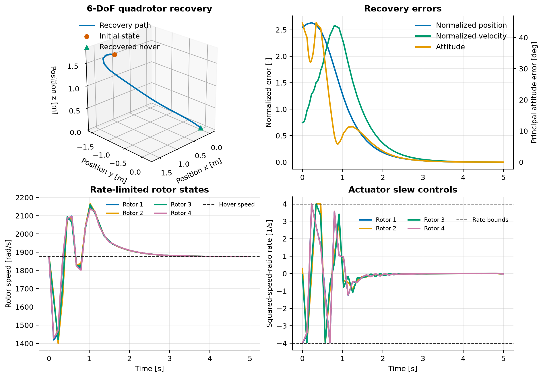
After solving, the script reconstructs all states and controls at 4,001 physical times. It converts the dimensionless rotor states back to physical speed, checks dense speed, slew-rate, and MRP-chart bounds, and verifies the optimized terminal state against the phase endpoint. It separately requires small terminal position, velocity, attitude, and angular-rate errors; all four commands equal to one; and small terminal linear and angular accelerations. The last checks distinguish a balanced hover from a trajectory that merely passes near zero state with an unbalanced terminal wrench.

Quantity	Default-solve value
Objective \(J\)	\(8.54936175\)
Terminal position error	\(0.000001\ \mathrm m\)
Terminal velocity error	\(0.000002\ \mathrm{m/s}\)
Terminal principal-attitude error	\(0.000089^\circ\)
Terminal angular-rate error	\(0.000000\ \mathrm{rad/s}\)
Maximum terminal rotor-command error	\(0\) at reported precision
Terminal linear-acceleration norm	\(1.532\times10^{-5}\ \mathrm{m/s^2}\)
Terminal angular-acceleration norm	\(3.843\times10^{-19}\ \mathrm{rad/s^2}\)
Dense rotor-speed range	\(1400.89\) to \(2164.74\ \mathrm{rad/s}\)
Peak squared-speed-ratio slew	\(4.0000\ \mathrm{s^{-1}}\)
Peak total thrust	\(0.4258\ \mathrm N\)
Minimum MRP-chart radial margin	\(0.569544\)

The optimizer therefore returns the vehicle close to rest with a balanced terminal rotor state, rather than only minimizing the kinematic state errors. The reconstructed rotor speeds and slew controls respect their dense limits. These figures describe a local optimum of the discretized problem, not a proof of a global optimum.

Source code

See the complete runnable example: examples/drone_stabilization.py.