Building HVAC Demand Management

Background

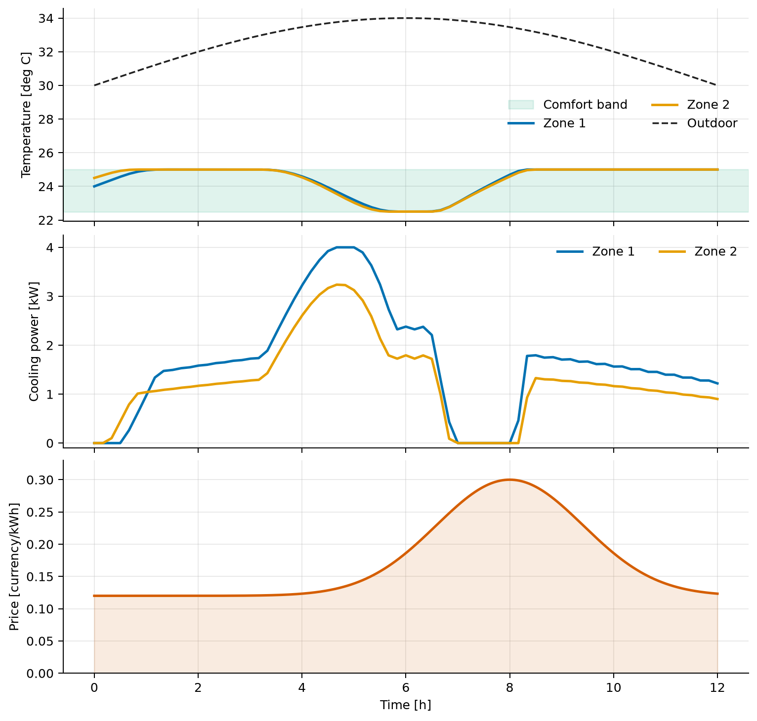
Commercial buildings can shift cooling electricity away from expensive hours by using the building's thermal mass. Pre-cooling is useful only while occupant comfort, equipment capacity, and the coupling between zones remain explicit. This example schedules two neighbouring office zones over a 12-hour day.

The model is intentionally small, but it retains the structure used in building energy management: resistance-capacitance thermal dynamics, internal heat gains, a coefficient of performance, time-varying weather and prices, and hard comfort bounds.

Problem formulation

Let \(T_i(t)\) be the temperature of zone \(i\in\{1,2\}\), \(P_i(t)\) its electrical cooling power, and \(j\ne i\) the neighbouring zone. The thermal balance is

\[ C_i\dot T_i =G_i\bigl(T_o(t)-T_i\bigr) +G_{12}(T_j-T_i)+Q_i-\eta P_i, \]

where \(C_i\) is thermal capacitance, \(G_i\) is outdoor conductance, \(G_{12}\) is inter-zone conductance, \(Q_i\) is the internal heat gain, and \(\eta\) is the cooling coefficient of performance. The exogenous profiles are

\[ T_o(t)=30+4\sin\!\left(\frac{\pi t}{12}\right), \qquad p(t)=0.12+0.18\exp\!\left[-\left(\frac{t-8}{2}\right)^2\right]. \]

The objective combines the time-of-use electricity charge with a small smooth control penalty:

\[ \min_{T_1,T_2,P_1,P_2} J=\int_0^{12} \left[p(t)(P_1+P_2)+\gamma(P_1^2+P_2^2)\right]\,\mathrm dt, \qquad \gamma=0.004. \]

The initial temperatures are fixed and the terminal temperatures are free:

\[ (T_1(0),T_2(0))=(24.0,24.5)\ ^\circ\mathrm C. \]

Comfort and actuator constraints apply throughout the horizon:

\[ 22.5\le T_i(t)\le25.0\ ^\circ\mathrm C, \qquad 0\le P_i(t)\le4.0\ \mathrm{kW}. \]

Parameters, variables, and units

Symbol	Meaning	Value or unit
\(t\)	Time from the start of the occupied period	h
\(T_1,T_2\)	Zone air temperatures	°C
\(P_1,P_2\)	Electrical cooling powers	kW
\(C_1,C_2\)	Zone thermal capacitances	\(4.0, 3.2\ \mathrm{kWh/K}\)
\(G_1,G_2\)	Outdoor conductances	\(0.55, 0.42\ \mathrm{kW/K}\)
\(G_{12}\)	Inter-zone conductance	\(0.18\ \mathrm{kW/K}\)
\(Q_1,Q_2\)	Internal heat gains	\(1.20, 0.80\ \mathrm{kW}\)
\(\eta\)	Cooling coefficient of performance	\(3.2\)
\(p(t)\)	Time-of-use electricity price	currency/kWh

Modeling choices

The controls are electrical powers; multiplying by the coefficient of performance converts them to removed thermal power. The quadratic term is a small regularizer that discourages unnecessarily sharp or opposing zone commands. Peak power is reported after the solve but is not a demand-charge term in this objective.

The implementation uses a \(72\times2\) Lobatto mesh. With two Lobatto points per interval, the reconstructed states and controls are piecewise linear, so a fine mesh resolves the smooth weather and price profiles while making dense bound checks straightforward. The terminal temperatures remain free because the problem represents one occupied scheduling window rather than a periodic day.

Run the example

python -m examples.building_hvac_control

Save the figure without opening a window:

python -m examples.building_hvac_control --save building-hvac-control.png --no-show

The script follows the common example pipeline:

system, phase = build_problem()
guess = initial_guess(phase)
solution = solve_problem(system, guess)
plot_solution(solution)

Verified result

The solver result is reconstructed at 4,001 uniformly spaced times. The script checks both zone temperatures and both cooling powers against their physical bounds, then independently integrates energy and energy charge.

Quantity	Verified value
Objective \(J\)	\(5.89133099\)
Cooling electricity	\(35.466949\ \mathrm{kWh}\)
Time-of-use energy charge	\(5.587746\) currency units
Peak total electrical power	\(7.237222\ \mathrm{kW}\)
Maximum dense path-bound violation	\(2.495\times10^{-7}\)

The small dense violation is below the script's \(2\times10^{-6}\) numerical tolerance. The optimal schedule pre-cools before the price peak and lets both temperatures rise within the comfort band while electricity is most expensive.

Source code

See the complete runnable example: examples/building_hvac_control.py.