Battery Energy Arbitrage

Background

A grid-connected battery can buy electricity when prices are low and return it when prices are high. A useful dispatch model must account for conversion losses, an operating state-of-charge window, finite charge and discharge power, cycling wear, and the value of energy left in the battery at the end of the day.

This example optimizes one 24-hour schedule for a nominal 100 kWh battery. It uses separate nonnegative charge and discharge controls so that the dynamics and objective remain smooth when power changes direction.

Problem formulation

Let \(E(t)\) be stored energy, \(P_c(t)\) charging power drawn from the grid, and \(P_d(t)\) discharge power delivered to the grid. With charge and discharge efficiencies \(\eta_c\) and \(\eta_d\),

\[ \dot E=\eta_cP_c-\frac{P_d}{\eta_d}. \]

The smooth day-ahead price profile is

\[ \begin{aligned} p(t)={}&0.12 +0.08\exp\!\left[-\left(\frac{t-8}{2}\right)^2\right] +0.22\exp\!\left[-\left(\frac{t-19}{2.4}\right)^2\right]\\ &-0.06\exp\!\left[-\left(\frac{t-13}{2.5}\right)^2\right]. \end{aligned} \]

The optimizer minimizes grid cash flow plus a convex cycling proxy:

\[ \min_{E,P_c,P_d}J=\int_0^{24} \left[p(t)(P_c-P_d)+\gamma(P_c^2+P_d^2)\right]\,\mathrm dt, \qquad \gamma=0.003. \]

A negative first term represents net market revenue. The terminal-energy condition prevents the optimizer from treating the initial inventory as free energy:

\[ E(0)=E(24)=50\ \mathrm{kWh}. \]

The operating and power bounds are

\[ 10\le E(t)\le90\ \mathrm{kWh}, \qquad 0\le P_c(t),P_d(t)\le20\ \mathrm{kW}. \]

Parameters, variables, and units

Symbol	Meaning	Value or unit
\(t\)	Time	h
\(E\)	Stored energy	kWh
\(P_c,P_d\)	Charge and discharge powers	kW
\(p(t)\)	Day-ahead electricity price	currency/kWh
\(E_{\mathrm{nom}}\)	Nominal energy capacity	\(100\ \mathrm{kWh}\)
\(\eta_c\)	Charge efficiency	\(0.95\)
\(\eta_d\)	Discharge efficiency	\(0.94\)
\(\gamma\)	Quadratic cycling-cost weight	\(0.003\) currency/(kW² h)

Modeling choices

Separate charge and discharge controls avoid the nondifferentiability of a single signed-power efficiency model. No nonconvex complementarity constraint \(P_cP_d=0\) is imposed. For this price profile, conversion losses and the positive quadratic penalty already make simultaneous charging and discharging uneconomic; the dense validation reports the residual overlap explicitly.

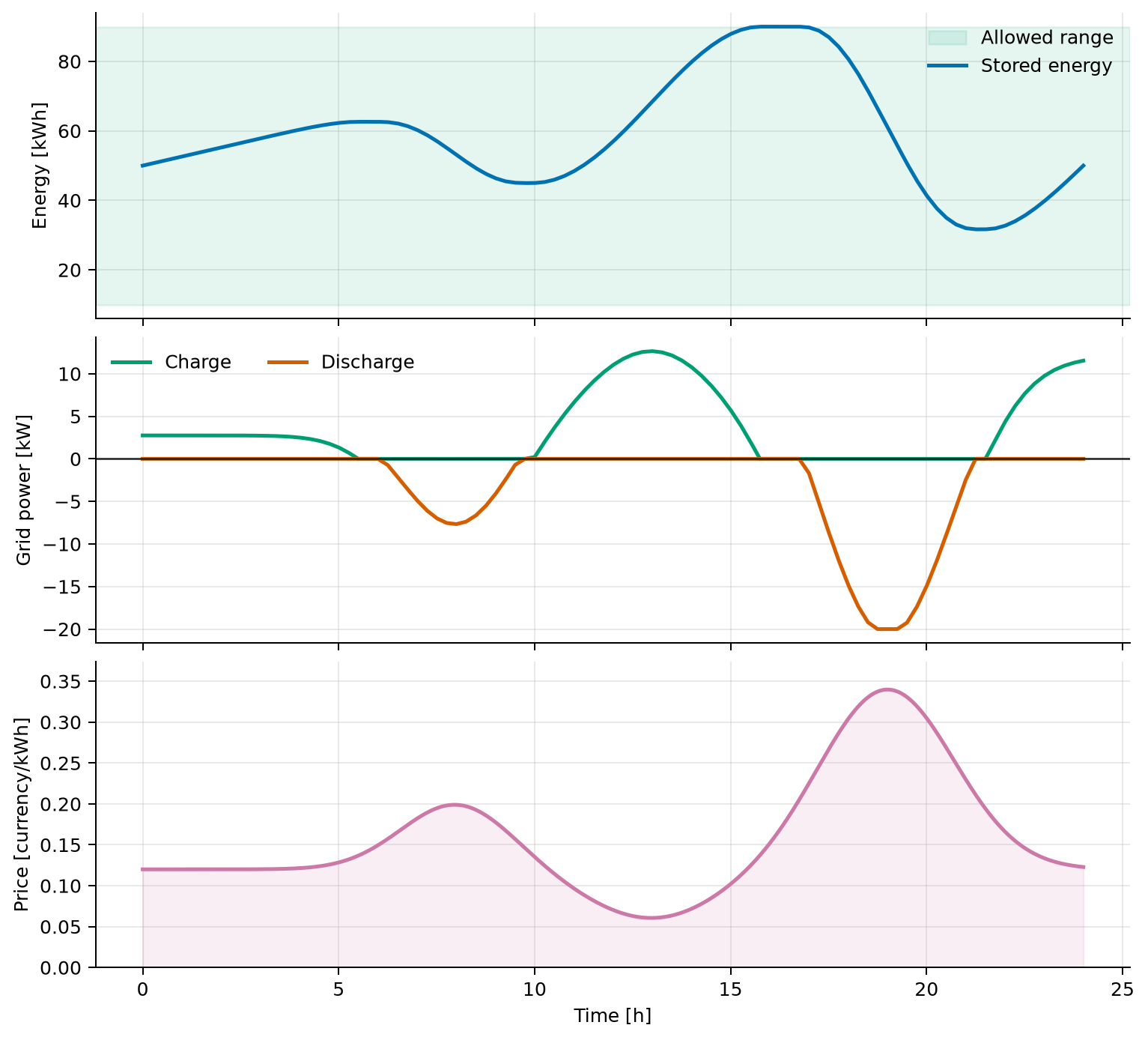
The 10--90 kWh operating window leaves reserve at both ends of the nominal capacity. Equal initial and terminal energy makes daily cash flows comparable. The model uses a \(96\times2\) Lobatto mesh, producing piecewise-linear state and power histories over 15-minute intervals.

Run the example

python -m examples.battery_energy_arbitrage

Save the figure without opening a window:

python -m examples.battery_energy_arbitrage --save battery-energy-arbitrage.png --no-show

The implementation follows the common composable pipeline:

system, phase = build_problem()
guess = initial_guess(phase)
solution = solve_problem(system, guess)
plot_solution(solution)

Verified result

The script reconstructs stored energy and both powers at 4,001 times, checks all bounds and the terminal inventory, and independently integrates market cash flow and battery throughput.

Quantity	Verified value
Objective \(J\)	\(-7.36173187\) currency units
Energy-market cash flow	\(-12.312375\) currency units
Battery throughput \(\int(P_c+P_d)\,\mathrm dt\)	\(151.426069\ \mathrm{kWh}\)
Maximum simultaneous charge/discharge	\(5.799\times10^{-8}\ \mathrm{kW}\)
Maximum dense path-bound violation	\(8.949\times10^{-7}\)

The objective is less negative than the market cash flow because it includes the positive cycling penalty. The battery charges around low-price periods and discharges into the two price peaks; the largest dense bound error remains below the \(2\times10^{-6}\) validation tolerance.

Source code

See the complete runnable example: examples/battery_energy_arbitrage.py.