Minimum-Time Variable-Inertia Robot Arm

Background

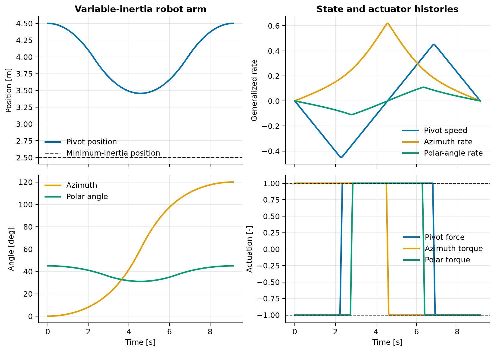
This benchmark represents a five-meter arm with a pivot that can slide along its length. Moving the pivot changes both rotational inertias. A time-optimal solution therefore does more than rotate the arm: it temporarily moves the pivot inward, reorients the arm while the inertia is lower, and returns the pivot to its required terminal position.

The model is useful for learning how a free final time, state-dependent equivalent inertia, and several saturated actuators are expressed in one Pockit phase. It is a deliberately decoupled teaching benchmark rather than a complete rigid-body manipulator model. In particular, it omits inertia-rate momentum terms such as \(\dot I(q)\dot q\), Coriolis terms, and the remaining couplings of a full rigid-body mass matrix.

Problem formulation

Let

\[ \boldsymbol{x} = \begin{bmatrix} r & v_r & \psi & \omega_\psi & \phi & \omega_\phi \end{bmatrix}^{\mathsf T}, \qquad \boldsymbol{u} = \begin{bmatrix} u_r & u_\psi & u_\phi \end{bmatrix}^{\mathsf T}. \]

Here \(r\) is the pivot position along an arm of length \(L=5\), \(\psi\) is the azimuth about a fixed axis, and \(\phi\) is the polar angle measured from that axis. The scaled polar-angle and azimuth inertias are

\[ I_\phi(r)=\frac{(L-r)^3+r^3}{3}, \qquad I_\psi(r,\phi)=I_\phi(r)\sin^2\phi. \]

The dynamics are

\[ \begin{aligned} \dot r &= v_r, & \dot v_r &= \frac{u_r}{L},\\ \dot\psi &= \omega_\psi, & \dot\omega_\psi &= \frac{u_\psi}{I_\psi(r,\phi)},\\ \dot\phi &= \omega_\phi, & \dot\omega_\phi &= \frac{u_\phi}{I_\phi(r)}. \end{aligned} \]

The objective is minimum time:

\[ \min_{\boldsymbol{x},\boldsymbol{u},t_f} \quad t_f =\int_0^{t_f}1\,\mathrm dt. \]

The generalized coordinates stay in their physical chart,

\[ 0\le r\le L, \qquad \delta\le\phi\le\pi-\delta, \qquad \delta=10^\circ. \]

The polar-angle margin keeps \(I_\psi\) away from the coordinate singularities at \(\phi=0\) and \(\phi=\pi\). All three actuator commands are bounded,

\[ -1\le u_r,u_\psi,u_\phi\le1, \]

and the endpoint conditions are

\[ \boldsymbol{x}(0) = \begin{bmatrix} 4.5&0&0&0&\pi/4&0 \end{bmatrix}^{\mathsf T}, \]

\[ \boldsymbol{x}(t_f) = \begin{bmatrix} 4.5&0&2\pi/3&0&\pi/4&0 \end{bmatrix}^{\mathsf T}. \]

The initial time is fixed at zero and \(t_f\) is an optimization variable.

Variables and units

The benchmark uses SI-like coordinates with scaled inertias and actuator commands.

Symbol	Meaning	Unit
\(t\)	Time	s
\(r\)	Pivot position along the arm	m
\(v_r\)	Pivot speed	m/s
\(\psi,\phi\)	Azimuth and polar angles	rad
\(\omega_\psi,\omega_\phi\)	Angular rates	rad/s
\(I_\psi,I_\phi\)	Scaled rotational inertias	scaled
\(u_r,u_\psi,u_\phi\)	Bounded actuator commands	-

Modeling choices

The state order alternates each generalized coordinate with its rate, which makes the second-order structure visible in the equivalent model. The polar angle is a state, not a fixed parameter: even though its initial and terminal values are both \(\pi/4\), the optimizer may move it temporarily to alter the azimuth inertia. These equations should not be interpreted as a momentum-consistent derivation for a physical sliding-pivot arm; such a model would require the omitted \(\dot I\dot q\) and coupled rigid-body terms.

The phase uses 160 Lobatto mesh intervals with two points per interval. Each control is therefore piecewise linear, so actuator bounds imposed at the two endpoints hold everywhere inside the interval; a high-order polynomial could overshoot between constrained nodes. Ipopt's bound relaxation is disabled, and the returned states and controls are independently evaluated with V_x and V_u at 10,001 times. This dense check rejects non-finite values and violations of either the physical coordinate domain or the actuator limits. Only the actuator limits are marked as bang-bang constraints.

The initial guess sets \(t_f=10.5\ \mathrm{s}\), reverses the azimuth torque halfway through the maneuver, and suggests moving the pivot inward before returning it. This gives Ipopt a useful scale without prescribing the solution.

Run the example

From the repository root, run:

python -m examples.robot_arm

To save the plot without opening an interactive window:

python -m examples.robot_arm --save robot-arm.png --no-show

Key implementation

import numpy as np
import sympy as sp

from pockit.lobatto import System

system = System(0)
phase = system.new_phase(
    [
        "pivot_position",
        "pivot_speed",
        "azimuth",
        "azimuth_rate",
        "polar_angle",
        "polar_angle_rate",
    ],
    ["pivot_force", "azimuth_torque", "polar_torque"],
)
r, v_r, _, omega_psi, phi, omega_phi = phase.x
u_r, u_psi, u_phi = phase.u

I_phi = ((5.0 - r) ** 3 + r**3) / 3.0
I_psi = I_phi * sp.sin(phi) ** 2
phase.set_dynamics(
    [v_r, u_r / 5.0, omega_psi, u_psi / I_psi, omega_phi, u_phi / I_phi]
)
phase.set_integral([1.0])
polar_margin = np.deg2rad(10.0)
phase.set_phase_constraint(
    [r, phi, u_r, u_psi, u_phi],
    [0.0, polar_margin, -1.0, -1.0, -1.0],
    [5.0, np.pi - polar_margin, 1.0, 1.0, 1.0],
    [False, False, True, True, True],
)
phase.set_boundary_condition(
    [4.5, 0.0, 0.0, 0.0, 0.25 * np.pi, 0.0],
    [4.5, 0.0, 2.0 * np.pi / 3.0, 0.0, 0.25 * np.pi, 0.0],
    0.0,
    None,
)
phase.set_discretization(160, 2)
system.set_phase([phase])
system.set_objective(phase.I[0])

The complete script also constructs the initial guess, solves with bound_relax_factor=0.0, checks the Ipopt return status and endpoint values, and rejects a solution if any of 10,001 state or control samples is non-finite or leaves its stated domain.

Verified result

With the default mesh and Ipopt settings, the example converges to

\[ t_f=9.141679261\ \mathrm{s}. \]

The smallest pivot position is \(3.455698\ \mathrm{m}\). It does not reach the minimum-inertia location \(L/2=2.5\ \mathrm{m}\): moving farther inward would reduce rotational inertia but would cost more transfer time. The actuator histories show the expected saturated arcs and linear transitions between them. On the 10,001-point check grid, the complete interpolated control range is \([-0.999999996,0.999999996]\), inside the required \([-1,1]\) bounds. The smallest polar angle is \(31.099876^\circ\), comfortably above the \(10^\circ\) singularity margin, and the maximum physical-domain violation is zero to the reported precision.

Source code

See the complete runnable example: examples/robot_arm.py.