Humanoid Centroidal Motion Retargeting
Background
Motion retargeting maps a recorded or designed human motion to a robot with different proportions. Scaling positions by leg length gives a useful kinematic reference, but it does not make that reference satisfy the robot's Newton-Euler equations or contact limits.
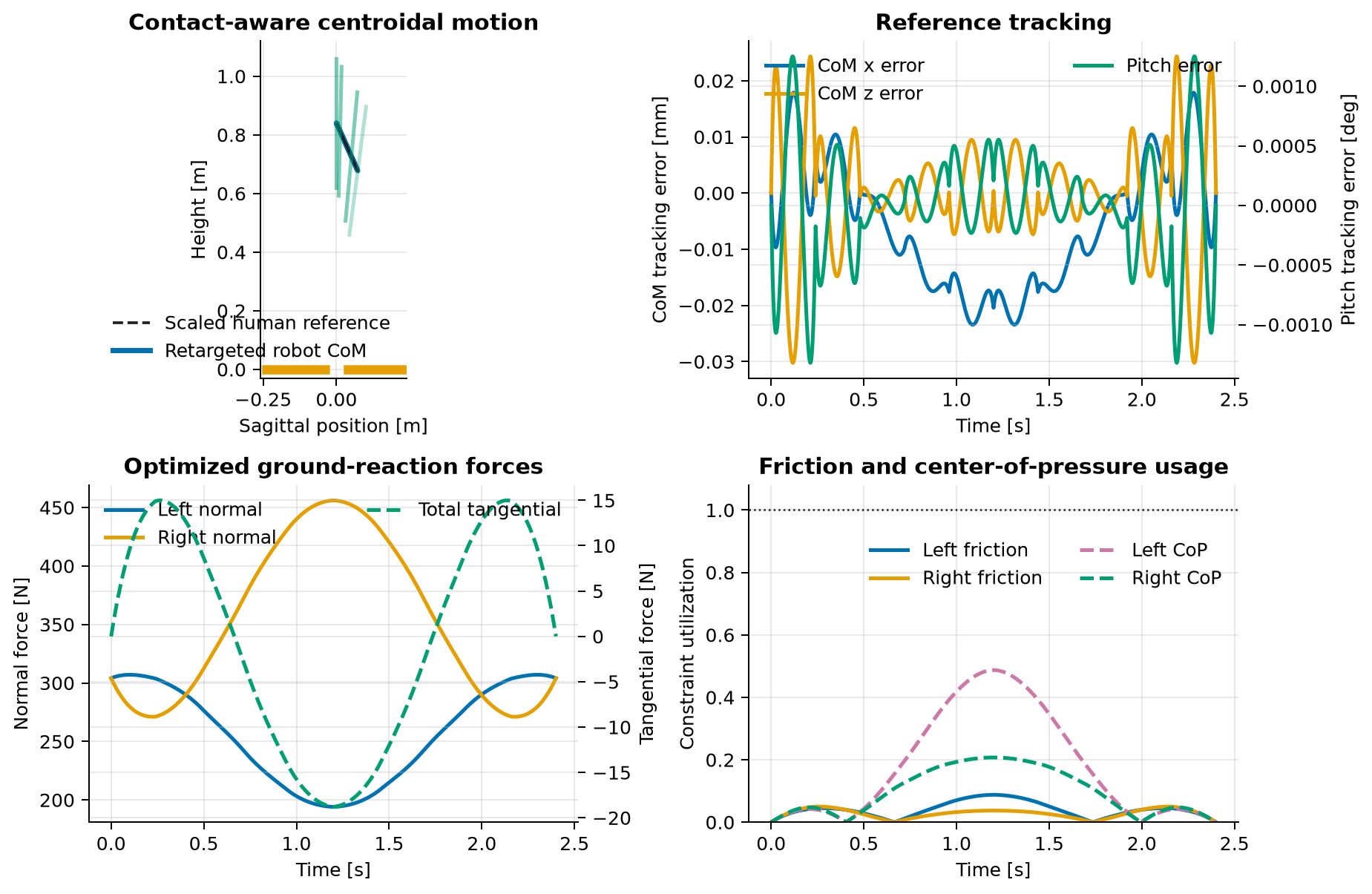
This example treats the entire known squat-and-reach reference as a preview. It optimizes the planar center-of-mass (CoM) trajectory, body pitch, and both foot contact wrenches over the full horizon. Tracking terms keep the result close to the scaled human motion, while centroidal dynamics, unilateral contact, Coulomb friction, center-of-pressure (CoP), wrench, and wrench-rate constraints make it dynamically consistent within the reduced model.
Geometrically scaled reference
The fixed horizon is \(T=2.4\ \mathrm{s}\). With normalized time \(\tau=t/T\), define the rest-to-rest, \(C^2\) bump
Its first two derivatives are
The leg-length scale is
The desired CoM position, velocity, pitch, and pitch rate are
Thus the scaled reference moves forward by \(0.072604\ \mathrm m\), squats by \(0.162292\ \mathrm m\), and reaches \(0.13\ \mathrm{rad}\) pitch at the midpoint. The reference acceleration is used to construct a balanced initial wrench guess; it is not imposed as a trajectory constraint.
State, control, and units
Let \(i\in\{L,R\}\) identify the left and right feet. The state and control are
| Symbol | Meaning | Unit or value |
|---|---|---|
| \(c_x,c_z\) | Sagittal CoM position and height | m |
| \(v_x,v_z\) | CoM velocity | m/s |
| \(\theta,\omega\) | Body pitch and pitch rate | rad, rad/s |
| \(f_{ix},f_{iz}\) | Ground-on-robot tangential and normal force | N |
| \(m_i\) | Foot contact moment about the out-of-plane axis | \(\mathrm{N\,m}\) |
| \(\dot f_{ix},\dot f_{iz},\dot m_i\) | Contact-wrench rates | \(\mathrm{N/s}\), \(\mathrm{N\,m/s}\) |
| \(M\) | Robot mass | \(62\ \mathrm{kg}\) |
| \(I_y\) | Constant centroidal pitch inertia | \(8\ \mathrm{kg\,m^2}\) |
| \(g\) | Gravitational acceleration | \(9.81\ \mathrm{m/s^2}\) |
| \(a\) | Foot-center offset; centers are at \(x=\pm a\) | \(0.14\ \mathrm m\) |
| \(\ell\) | Foot half-length | \(0.10\ \mathrm m\) |
| \(\mu\) | Coulomb friction coefficient | \(0.55\) |
Centroidal dynamics
The feet are fixed at \((-a,0)\) and \((a,0)\). Translational dynamics are
Pitch evolves according to
The six remaining state equations are the wrench integrators
Tracking and regularization objective
Define the tracking errors and normalization scales as
The normalized contact-wrench vector is
Each component of the normalized rate \(\overline{\boldsymbol u}\) is the corresponding control divided by its rate limit. The objective is
Wrench regularization favors approximately even static support without fixing the force split. Rate regularization produces smooth contact histories.
Contact and path constraints
The normal-force limit is
For each foot, unilateral contact, the planar Coulomb cone, and the CoP bound are
The last inequality keeps the resultant CoP within the \(0.20\ \mathrm m\) foot support length. Additional component bounds are
The centroidal state bounds are
For each foot, wrench-rate bounds are
Boundary conditions
Both endpoints are the same symmetric static-support state:
at \(t=0\) and \(t=T\).
Numerical method and independent validation
The default problem uses a \(10\times4\) Lobatto mesh. The initial guess follows the scaled reference and distributes the dynamically required wrench between the feet with zero foot moments. Pockit then optimizes all states and wrench rates simultaneously.
After solving, the script reconstructs the trajectory at 4,001 times and
checks state, wrench-rate, friction, and CoP constraints. It also fits cubic
splines to the optimized wrench rates and independently integrates all 12
continuous states with solve_ivp using \(\mathrm{rtol}=2\times10^{-9}\) and
\(\mathrm{atol}=2\times10^{-11}\). Force errors are scaled by \(Mg\), moment
errors by \(Mg\ell\), and the first six state errors by their native unit
scales before taking the maximum.
Verified result
| Quantity | Verified value |
|---|---|
| RMS CoM \(x\) tracking error | \(0.012\ \mathrm{mm}\) |
| RMS CoM \(z\) tracking error | \(0.010\ \mathrm{mm}\) |
| RMS pitch tracking error | \(0.0005^\circ\) |
| Minimum friction margin (\mu f_z- | f_x |
| Minimum CoP margin (\ell f_z- | m |
| Maximum dense state-bound violation | \(0\) |
| Maximum independently integrated scaled mismatch | \(4.933\times10^{-4}\) |
The strictly positive contact margins show that neither friction nor CoP is active in this local optimum. They do not certify feasibility for a full joint-level humanoid model.
Scope and limitations
This example performs planar centroidal preview and retargeting only. It uses fixed feet, a constant pitch inertia, and continuous double support. It does not model joint coordinates or torques, kinematic reachability, self-collision, actuator limits, link inertia variation, contact switching, three-dimensional friction, or balance under disturbances.
The optimized CoM, pitch, and foot-wrench histories must therefore be passed to a downstream whole-body inverse-kinematics or trajectory-optimization stage that enforces the robot's complete multibody and collision constraints.
Run the example
Save the figure without opening a window:
The optional --quick flag uses a smaller \(8\times3\) mesh for a faster
smoke test. The verified values above use the default mesh.
system, phase = build_problem()
guess = initial_guess(phase)
solution = solve_problem(system, guess)
plot_solution(solution)
Source code
See the complete runnable example:
examples/humanoid_motion_retargeting.py.