Optimal Irrigation Scheduling with a Root-Zone Water Balance

Background

An irrigation scheduler must protect a crop during dry periods without applying unnecessary water. Rainfall, crop demand, soil storage, and drainage all vary over time, while a real valve cannot change flow instantaneously. This example uses a 14-day weather forecast to trade applied water against a smooth proxy for water-stress-related yield loss.

The state is plant-available water above the wilting point. A hard storage reserve prevents severe depletion; a soft stress penalty distinguishes otherwise feasible schedules and encourages water to be supplied when it is most useful.

Problem formulation

Let \(S(t)\) be root-zone storage, \(i(t)\) irrigation rate, and \(u(t)=\dot i(t)\) the valve-ramp command. The forecast effective rainfall and potential crop evapotranspiration are

\[ R(t)=9\exp\!\left[-\left(\frac{t-3.8}{0.55}\right)^2\right] +4\exp\!\left[-\left(\frac{t-10.4}{0.75}\right)^2\right], \]

\[ ET_p(t)=5.2+0.8\sin\!\left(\frac{2\pi(t-1)}{7}\right). \]

The smooth extraction factor

\[ f(S)=\frac{S(C+S_{50})}{C(S+S_{50})} \]

is zero at the wilting point \(S=0\) and equals one at root-zone capacity \(S=C\). Actual evapotranspiration is \(ET_a=ET_p f(S)\). Deep percolation is modeled as

\[ D(S)=d_C\left(\frac{S}{C}\right)^6, \]

which rises sharply near capacity. The dynamics are therefore

\[ \dot S=R(t)+i-ET_p(t)f(S)-D(S), \qquad \dot i=u. \]

The dimensionless objective is

\[ \min_{S,i,u}\;J=\int_0^T \left[ w_i i+w_s(1-f(S))^2+w_u u^2 \right]\,\mathrm dt. \]

The first term prices applied water, the second is a yield-loss proxy based on water stress, and the third discourages rapid valve motion. It is not a mechanistic crop-yield equation.

Endpoint and path constraints are

\[ S(0)=S(T)=58\ \mathrm{mm}, \qquad i(0)=i(T)=0, \]

\[ 12\le S(t)\le110\ \mathrm{mm}, \qquad 0\le i(t)\le10\ \mathrm{mm\,day^{-1}}, \]

\[ |u(t)|\le8\ \mathrm{mm\,day^{-2}}. \]

Variables, parameters, and units

Symbol	Meaning	Value or unit
\(t\)	Time	days
\(S\)	Plant-available root-zone storage above wilting	mm
\(i\)	Irrigation rate	mm/day
\(u=\dot i\)	Irrigation ramp	mm/day²
\(R\)	Effective rainfall	mm/day
\(ET_p,ET_a\)	Potential and actual evapotranspiration	mm/day
\(D\)	Deep percolation	mm/day
\(C\)	Root-zone capacity	\(110\) mm
\(S_{50}\)	Michaelis-Menten storage scale before normalization at \(C\)	\(24\) mm
\(d_C\)	Percolation at capacity	\(2.2\) mm/day
\(w_i\)	Irrigation weight	\(0.030\) mm⁻¹
\(w_s\)	Stress weight	\(1.0\) day⁻¹
\(w_u\)	Ramp weight	\(2.0\times10^{-4}\) day³/mm²

The implementation optimizes the scaled state \(S/C\) to improve numerical conditioning, while all equations and reported values here use physical water depth.

Modeling choices

Irrigation rate is a state rather than a directly discontinuous control. Optimizing its bounded derivative produces a continuous schedule and makes the zero-flow endpoint conditions meaningful. A \(140\times2\) Lobatto mesh uses piecewise-linear interpolation, which also preserves the nonnegative irrigation bound between nodes.

Equal initial and terminal storage makes total inflow and total loss comparable over the forecast window. It is a bookkeeping condition for this scheduling exercise, not evidence that the weather or crop state is periodic.

Independent validation

The dense reconstructed solution must satisfy the integrated water balance

\[ S(T)-S(0)=\int_0^T \left[R+i-ET_a-D\right]\,\mathrm dt, \]

and the actuator balance

\[ i(T)-i(0)=\int_0^T u(t)\,\mathrm dt. \]

The script independently evaluates both identities at 6,001 times, checks all state and actuator bounds, and reports the individual water-budget terms.

Verified result

Quantity	Verified value
Objective \(J\)	\(1.74128841\)
Total irrigation	\(50.888617\) mm
Effective rainfall	\(14.091008\) mm
Actual evapotranspiration	\(63.918972\) mm
Deep percolation	\(1.060678\) mm
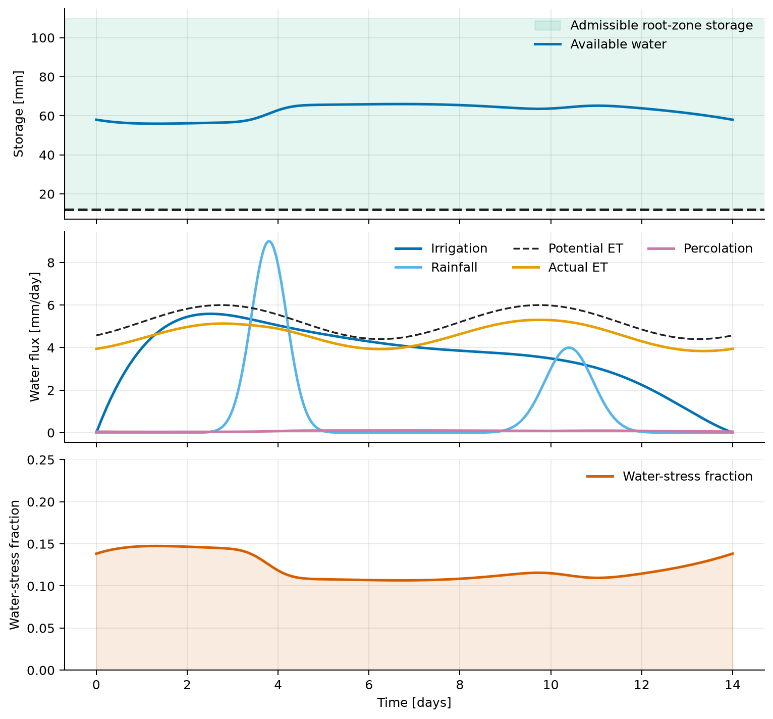
Minimum root-zone storage	\(55.962540\) mm
Dense water-balance error	\(2.437\times10^{-5}\) mm
Dense actuator-balance error	\(1.288\times10^{-6}\) mm/day
Maximum dense path-bound violation	\(0\)

The integrated inflow is \(50.888617+14.091008=64.979625\) mm and the integrated loss is \(63.918972+1.060678=64.979650\) mm; their small difference is consistent with the independently reported quadrature residual.

Scope and limitations

The calculation assumes a perfect deterministic weather forecast, a spatially uniform root zone, and continuously available irrigation. It omits runoff, application and conveyance losses, discrete irrigation windows, pump on/off logic, soil layers, and forecast uncertainty. The stress term is only a smooth yield proxy. Field scheduling requires calibrated soil-crop parameters and operational constraints.

Run the example

python -m examples.irrigation_scheduling

Save the figure without opening a window:

python -m examples.irrigation_scheduling --save irrigation-scheduling.png --no-show

system, phase = build_problem()
guess = initial_guess(phase)
solution = solve_problem(system, guess)
plot_solution(solution)

Source code

See the complete runnable example: examples/irrigation_scheduling.py.