Training an Augmented Neural ODE on XOR

Background

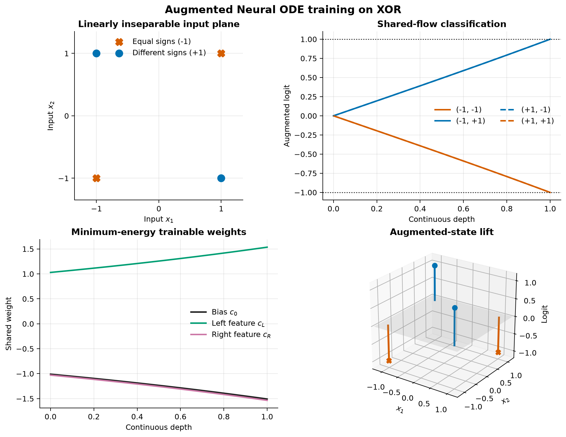
The XOR data set contains four corners of a square. Points whose coordinates have different signs belong to class \(+1\); points with equal signs belong to class \(-1\). No affine separator can give all four points a positive margin. An augmented Neural ODE can lift the samples into an additional state dimension where a fixed sign readout separates them.

This example formulates training as optimal control. Continuous-depth weights are the controls, the four sample logits are states, and hard endpoint constraints enforce classification. The architecture is intentionally restricted so its minimum-energy solution can also be derived analytically.

Data and architecture

The four fixed training samples and labels are

\[ \begin{array}{c|c} (x_1,x_2)&y\\ \hline (-1,-1)&-1\\ (-1,+1)&+1\\ (+1,-1)&+1\\ (+1,+1)&-1 \end{array}. \]

For sample \(i\), the augmented state is \((x_{1,i},x_{2,i},h_i)\). The input coordinates remain fixed:

\[ \dot x_{1,i}=0, \qquad \dot x_{2,i}=0. \]

Define the three fixed features

\[ \boldsymbol\phi_i= \begin{bmatrix} 1\\ \tanh\!\left(k(x_{1,i}+x_{2,i}+1)\right)\\ \tanh\!\left(k(x_{1,i}+x_{2,i}-1)\right) \end{bmatrix}, \qquad k=2. \]

All four samples share the trainable output-weight vector

\[ \boldsymbol c(t)=\begin{bmatrix}c_0(t)&c_L(t)&c_R(t)\end{bmatrix}^{\mathsf T}. \]

The leaky logit dynamics over continuous depth \(0\le t\le T=1\) are

\[ \dot h_i=\boldsymbol\phi_i^{\mathsf T}\boldsymbol c(t)-\lambda h_i, \qquad h_i(0)=0, \qquad \lambda=0.4. \]

Classification uses the fixed readout \(\operatorname{sign}(h_i(T))\).

Optimal-control problem

Training minimizes integrated squared weight magnitude:

\[ \min_{\boldsymbol c}\;J= \int_0^T\lVert\boldsymbol c(t)\rVert_2^2\,\mathrm dt. \]

The terminal signed-margin constraints and dense path bounds are

\[ 1\le y_i h_i(T)\le2, \qquad i=1,\ldots,4, \]

\[ -1.05\le x_{1,i}(t),x_{2,i}(t)\le1.05, \qquad |h_i(t)|\le2, \qquad |c_0(t)|,|c_L(t)|,|c_R(t)|\le3. \]

Each input state starts at its corresponding training coordinate. Its zero dynamics then keep that coordinate unchanged throughout the network depth; the \(\pm1.05\) bounds are numerical guardrails around the exact values \(\pm1\).

The implementation represents each terminal logit as a static parameter and links it to the phase endpoint. This makes the signed terminal inequalities ordinary system constraints.

Variables and units

Symbol	Meaning	Unit or value
\(t\)	Continuous network depth	dimensionless, \([0,1]\)
\(x_{1,i},x_{2,i}\)	Fixed input coordinates	dimensionless
\(h_i\)	Augmented logit for sample \(i\)	dimensionless
\(\boldsymbol\phi_i\)	Fixed nonlinear feature vector	dimensionless
\(c_0,c_L,c_R\)	Shared trainable output weights	dimensionless
\(k\)	Feature slope	\(2.0\)
\(\lambda\)	Latent-state leakage	\(0.4\)
\(J\)	Integrated squared-weight objective	dimensionless

Analytical optimum

Let \(F\in\mathbb R^{4\times3}\) contain the row vectors \(\boldsymbol\phi_i^{\mathsf T}\) and let \(\boldsymbol y\) contain the labels. For a prescribed terminal logit vector \(\boldsymbol h(T)\), define

\[ \boldsymbol a=F^+\boldsymbol h(T), \]

where \(F^+\) is the Moore-Penrose pseudoinverse. The squared norm of the terminal leakage kernel is

\[ K_\lambda=\int_0^T e^{-2\lambda(T-t)}\,\mathrm dt =\frac{1-e^{-2\lambda T}}{2\lambda}. \]

The minimum-energy weight history that realizes the terminal logits is

\[ \boldsymbol c^*(t)= \frac{\boldsymbol a}{K_\lambda}e^{-\lambda(T-t)}. \]

Symmetry and the energy objective make the lower margin active, so \(\boldsymbol h(T)=\boldsymbol y\). The analytical objective is therefore

\[ J^*=\frac{\lVert F^+\boldsymbol y\rVert_2^2}{K_\lambda} =4.8117131077. \]

This reference is computed independently of the collocation solution and is also used to form a well-scaled initial guess.

Modeling choices

The added scalar \(h_i\) supplies the dimension needed to separate XOR, while the original input coordinates are kept constant to make that lift visible. Only three shared output weights are trained. The tanh feature locations, feature slope, leakage, four inputs, and final sign readout are fixed.

A \(32\times4\) Lobatto mesh represents the smooth weight histories. After optimization, the script reconstructs all states and controls at 4,001 depths and independently integrates the learned vector field with a high-accuracy ODE solver.

Independent validation

The dense reconstruction checks input-coordinate drift, terminal linkage to the four static logits, signed margins, logit bounds, and weight bounds. A separate DOP853 solve then propagates all four logits from zero using the optimized shared weights. The script compares that forward trajectory with the collocation states.

As a second independent reference, it evaluates the closed-form weights and logits derived above at the same 4,001 depths and compares both trajectories and the objective with the numerical optimum.

Verified result

Quantity	Verified value
Numerical training objective	\(4.8117130115\)
Analytical objective	\(4.8117131077\)
Training accuracy on the four XOR points	\(100\%\)
Minimum signed terminal margin	\(0.9999999900\)
Maximum weight magnitude	\(1.5356236514\)
Maximum forward-reintegration error	\(5.471\times10^{-11}\)
Maximum analytical logit error	\(9.997\times10^{-9}\)

The objective differs from the analytical value by about \(9.62\times10^{-8}\), and the learned weights stay well inside their bound.

Scope and limitations

This is a training and transcription benchmark, not a general Neural ODE architecture. The fixed features explicitly encode the symmetry of these four XOR points, and only their shared output weights are learned. There is no held- out data, noise, parameter uncertainty, robustness test, or generalization claim. A practical classifier would learn a richer vector field and be evaluated on separate validation and test sets.

Run the example

python -m examples.neural_ode_xor

Save the figure without opening a window:

python -m examples.neural_ode_xor --save neural-ode-xor.png --no-show

system, phase = build_problem()
guess = initial_guess(phase)
solution = solve_problem(system, guess)
plot_solution(solution)

Source code

See the complete runnable example: examples/neural_ode_xor.py.