Energy-Optimal Wireless Transmission by Water Filling

Background

A transmitter with a hard deadline should avoid spending equal power at every instant when channel quality changes predictably. More data can be sent per joule during favorable channel conditions, but the complete payload must still arrive before the deadline and transmit power is bounded.

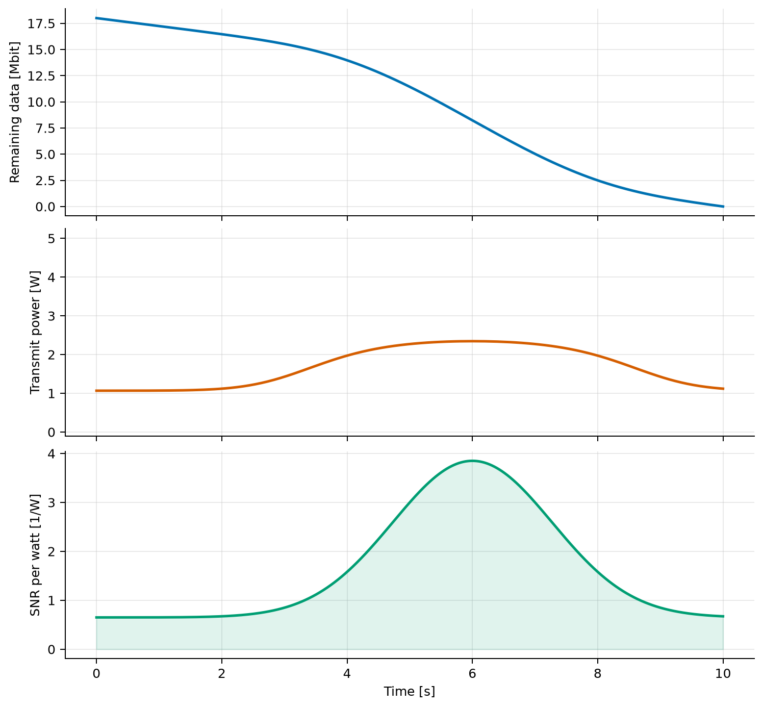
This example represents a receiver passing an access point: channel quality improves, reaches a peak, and then fades. The optimal-control result is checked against the classical water-filling allocation computed independently with a scalar root solve.

Problem formulation

Let \(q(t)\) be the remaining data and \(P(t)\) transmit power. The received SNR per watt is prescribed as

\[ g(t)=0.65+3.2\exp\!\left[-\left(\frac{t-6}{1.8}\right)^2\right] \quad [\mathrm{W}^{-1}]. \]

Using a Shannon-rate model with bandwidth \(B=1\) MHz gives

\[ R(t)=B\log_2\!\left(1+g(t)P(t)\right) \quad [\mathrm{Mbit\,s^{-1}}]. \]

The remaining-data dynamics are

\[ \dot q(t)=-R(t). \]

For a payload \(D=18\) Mbit and deadline \(T=10\) s, the endpoint conditions are

\[ q(0)=D, \qquad q(T)=0. \]

The objective and path constraints are

\[ \min_{q,P}\;E=\int_0^T P(t)\,\mathrm dt, \]

\[ 0\le q(t)\le D, \qquad 0\le P(t)\le P_{\max}=5\ \mathrm W. \]

Variables, parameters, and units

Symbol	Meaning	Value or unit
\(t\)	Time	s
\(q\)	Data remaining before the deadline	Mbit
\(P\)	Transmit power	W
\(g\)	Received SNR per watt	W⁻¹
\(R\)	Information rate	Mbit/s
\(B\)	Channel bandwidth	\(1\) MHz
\(D\)	Required payload	\(18\) Mbit
\(T\)	Transmission deadline	\(10\) s
\(P_{\max}\)	Power limit	\(5\) W
\(E\)	Transmit energy	J

Clipped water-filling reference

The terminal condition is equivalent to the integral payload constraint

\[ \int_0^T B\log_2(1+gP)\,\mathrm dt=D. \]

Applying the KKT stationarity condition to energy minimization gives the unconstrained positive-power relation

\[ P(t)=\nu-\frac{1}{g(t)}, \]

where \(\nu\) is a constant water level. Including both power bounds gives

\[ P_{\mathrm{wf}}(t)= \operatorname{clip}\!\left( \nu-\frac{1}{g(t)},\,0,\,P_{\max} \right). \]

The reference calculation uses Brent's method to choose \(\nu\) so that the dense-grid payload integral equals 18 Mbit. It does not use the Pockit trajectory, so agreement is an independent optimality check rather than a restatement of the collocation constraints.

Modeling choices

Remaining data is a state, making the delivery deadline an explicit terminal condition. The queue bounds also rule out sending more than the payload and then compensating mathematically. A \(100\times2\) Lobatto mesh uses piecewise- linear interpolation, which preserves the nonnegative queue and power bounds between nodes.

The deterministic channel profile is known over the entire horizon. This is an offline scheduling assumption; it is stronger than causal channel-state information available in many communication systems.

Independent validation

At 4,001 times, the script reconstructs \(q\) and \(P\), computes rate, and forms cumulative delivered data by numerical quadrature. It checks the queue identity

\[ q(t)=D-\int_0^t R(\tau)\,\mathrm d\tau \]

throughout the horizon, not just at \(T\). It then constructs the clipped water-filling reference, compares the full power histories and energies, and checks all dense path bounds.

Verified result

Quantity	Verified value
Transmit energy	\(16.97876379\) J
Delivered payload by dense quadrature	\(18.00004347\) Mbit
Analytical water level \(\nu\)	\(2.60489943\) W
Maximum water-filling power error	\(5.779\times10^{-4}\) W
Maximum cumulative queue-balance error	\(1.978\times10^{-3}\) Mbit
Maximum dense path-bound violation	\(0\)

The schedule raises power around the channel-quality peak and uses less power when the link is poor. The independent clipped water-filling result matches the optimized power within \(0.6\) mW over the dense grid.

Scope and limitations

The model assumes a deterministic perfectly known channel, a Shannon capacity rate law, continuous power control, and no coding delay. It omits circuit and idle power, interference, packetization, retransmissions, latency for individual packets, discrete modulation and coding, channel-estimation error, and fading uncertainty. Those effects can materially change an implementable radio policy.

Run the example

python -m examples.wireless_data_transmission

Save the figure without opening a window:

python -m examples.wireless_data_transmission --save wireless-data-transmission.png --no-show

system, phase = build_problem()
guess = initial_guess(phase)
solution = solve_problem(system, guess)
plot_solution(solution)

Source code

See the complete runnable example: examples/wireless_data_transmission.py.