Flexible Space Telescope Slew and Vibration Suppression

Background

Large observatories are not perfectly rigid. Reaction-wheel acceleration can excite appendage, optical-bench, or instrument modes, leaving line-of-sight jitter after the nominal attitude maneuver ends. A useful slew must therefore reach the target angle and settle both the rigid body and the flexible mode before observation begins.

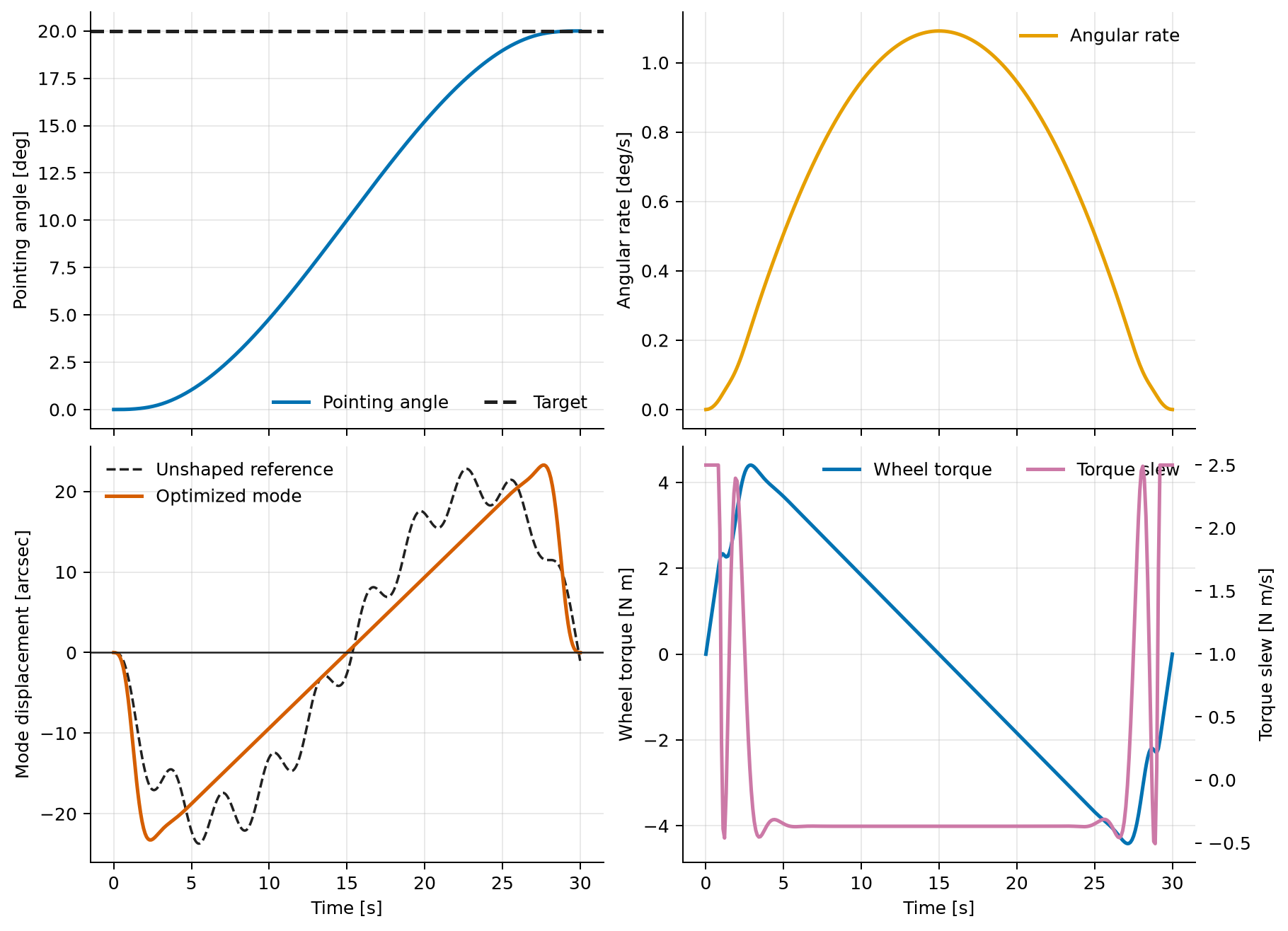
This example performs a \(20^\circ\) rest-to-rest slew in 30 seconds. Wheel torque is included as a state and its slew rate is the control, which makes actuator smoothness and endpoint unloading explicit.

Dynamic model

Let \(\theta\) be the rigid-body pointing angle, \(\omega=\dot\theta\) its rate, \(\eta\) an equivalent line-of-sight flexible displacement, \(\dot\eta\) its rate, \(\tau\) the reaction-wheel torque, and \(\nu=\dot\tau\) the commanded torque slew. A single lightly damped mode is coupled to rigid-body acceleration:

\[ \begin{aligned} \dot\theta&=\omega,\\ \dot\omega&=\frac{\tau}{J_s},\\ \dot\eta&=v_\eta,\\ \dot v_\eta &=-2\zeta_f\omega_fv_\eta-\omega_f^2\eta -b_f\frac{\tau}{J_s},\\ \dot\tau&=\nu. \end{aligned} \]

The fixed horizon and principal parameters are

\[ T=30\ \mathrm s,\qquad J_s=1800\ \mathrm{kg\,m^2},\qquad \omega_f=2\pi(0.32)\ \mathrm{rad/s}, \]

\[ \zeta_f=0.008,\qquad b_f=0.18. \]

The coupling coefficient maps rigid angular acceleration into the equivalent line-of-sight modal coordinate; it is an educational reduced-order model, not a finite-element telescope model.

Objective, endpoints, and path constraints

The normalized average cost penalizes wheel demand, torque slew, modal deflection, and modal velocity:

\[ \min J=\frac1T\int_0^T \left[ \left(\frac{\tau}{\tau_{\max}}\right)^2 +0.02\left(\frac{\nu}{\nu_{\max}}\right)^2 +0.8\left\{ \left(\frac{\eta}{\eta_s}\right)^2 +\left(\frac{v_\eta}{\omega_f\eta_s}\right)^2 \right\} \right]\,\mathrm dt, \]

with \(\tau_{\max}=12\ \mathrm{N\,m}\), \(\nu_{\max}=2.5\ \mathrm{N\,m/s}\), and \(\eta_s=10^{-4}\ \mathrm{rad}\). The endpoint conditions are

\[ \begin{aligned} (\theta,\omega,\eta,v_\eta,\tau)(0) &=(0,0,0,0,0),\\ (\theta,\omega,\eta,v_\eta,\tau)(T) &=(20^\circ,0,0,0,0). \end{aligned} \]

The path bounds are

\[ \begin{aligned} -0.02\ \mathrm{rad}&\le\theta(t) \le\frac{\pi}{9}+0.02\ \mathrm{rad},\\ |\omega(t)|&\le1.8^\circ/\mathrm s,\\ |\eta(t)|&\le8.0\times10^{-4}\ \mathrm{rad},\\ |v_\eta(t)|&\le\omega_f(8.0\times10^{-4})\ \mathrm{rad/s},\\ |\tau(t)|&\le12\ \mathrm{N\,m},\\ |\nu(t)|&\le2.5\ \mathrm{N\,m/s}. \end{aligned} \]

The angle bounds are written in radians in the implementation; \(\pi/9\ \mathrm{rad}=20^\circ\).

Variables and units

Symbol	Meaning	Unit
\(t\)	Maneuver time	s
\(\theta,\omega\)	Rigid pointing angle and angular rate	rad, rad/s
\(\eta,v_\eta\)	Equivalent line-of-sight mode displacement and rate	rad, rad/s
\(\tau\)	Reaction-wheel torque state	N m
\(\nu\)	Torque-slew control	N m/s
\(J_s\)	Rigid-body pointing inertia	kg m²
\(\omega_f,\zeta_f\)	Flexible-mode frequency and damping ratio	rad/s, dimensionless
\(b_f\)	Rigid-to-flexible acceleration coupling	dimensionless

Reference maneuver and independent checks

A quintic minimum-jerk rigid slew,

\[ \theta_{\mathrm{ref}}(t)=\theta_T \left(10s^3-15s^4+6s^5\right), \qquad s=t/T, \]

provides both the initial guess and an unshaped comparison. Its analytically defined angular acceleration is integrated through the flexible-mode equation independently of the optimizer.

For either trajectory, terminal modal amplitude is reported as

\[ A_f=\sqrt{\eta(T)^2+ \left(\frac{v_\eta(T)}{\omega_f}\right)^2}. \]

The optimized torque-slew samples are also linearly interpolated and all five physical differential equations are reintegrated with a high-accuracy DOP853 solver. This exposes discrepancies that a collocation endpoint check alone would hide.

Modeling choices and limits

Making torque a state and torque slew the control enforces continuous, rate-limited wheel demand and allows zero terminal torque. The \(300\times2\) Lobatto mesh resolves the 0.32 Hz mode while retaining piecewise-linear control histories.

Only one linear mode and one pointing axis are represented. The model omits wheel-speed and momentum capacity, wheel electrical dynamics, multiple structural modes, nonlinear geometry, sensor noise, disturbances, and a closed-loop attitude controller. The result demonstrates maneuver shaping; it is not a flight-qualified jitter prediction.

Run the example

python -m examples.flexible_telescope_slew

Save the figure without opening a window:

python -m examples.flexible_telescope_slew --save flexible-telescope-slew.png --no-show

Verified result

Quantity	Verified value
Objective \(J\)	\(0.41550448\)
Peak rigid angular rate	\(1.091275^\circ/\mathrm s\)
Peak wheel torque	\(4.414576\ \mathrm{N\,m}\)
Peak optimized flexible error	\(23.265178\ \mathrm{arcsec}\)
Unshaped terminal modal amplitude	\(5.276834\ \mathrm{arcsec}\)
Shaped, independently integrated terminal amplitude	\(0.1791\ \mathrm{arcsec}\)
Maximum scaled forward-integration error	\(1.708\times10^{-3}\)
Scaled forward endpoint error	\(9.845\times10^{-4}\)
Maximum integral-dynamics balance error	\(3.997\times10^{-15}\)

The collocation endpoint imposes zero modal displacement and velocity. The nonzero \(0.1791\) arcsec value is the stricter result obtained by independently integrating the interpolated command. It is about 3.4% of the unshaped minimum-jerk residual and remains below the script's 5% acceptance threshold.

Source code

See the complete runnable example: examples/flexible_telescope_slew.py.