Optimal Control of a Renewable Fishery

Background

A fishery manager must balance current catch against the biological stock that produces future catch. This example couples logistic biomass growth to a harvest schedule, then maximizes discounted dockside value while keeping the stock above an ecological floor. Changing the harvest rate also incurs a cost and is subject to an adjustment limit, so the result is an implementable smooth policy rather than an arbitrary sequence of catches.

The model is a finite-horizon planning benchmark. Matching the initial and terminal stock and harvest rate prevents simple end-of-horizon liquidation, but does not make the discounted solution an infinite-horizon periodic policy.

Problem formulation

Let \(B(t)\) denote aggregate biomass, \(H(t)\) the harvest rate, and \(u(t)\) the rate at which harvest is adjusted. Natural production follows logistic growth:

\[ G(B)=rB\left(1-\frac{B}{K}\right). \]

The state equations over \(0\le t\le T\) are

\[ \dot B=G(B)-H, \qquad \dot H=u. \]

The manager maximizes discounted net value

\[ \max_{B,H,u}\;V= \int_0^T e^{-\delta t} \left( pH-c\frac{H^2}{B}-a u^2 \right)\,\mathrm dt. \]

Here \(pH\) is dockside revenue, \(cH^2/B\) is a convex catch cost that rises as fish become scarce, and \(au^2\) discourages abrupt changes in fishing activity. Pockit minimizes the negative of this integral.

The endpoint conditions are cyclic in both states:

\[ B(0)=B(T)=680\ \mathrm{kt}, \qquad H(0)=H(T)=69.632\ \mathrm{kt\,year^{-1}}, \]

where the endpoint harvest equals natural growth at the initial biomass. The path constraints are

\[ 420\le B(t)\le1000\ \mathrm{kt}, \]

\[ 0\le H(t)\le105\ \mathrm{kt\,year^{-1}}, \qquad |u(t)|\le40\ \mathrm{kt\,year^{-2}}. \]

Variables, parameters, and units

Symbol	Meaning	Value or unit
\(t\)	Time	years
\(B\)	Aggregate fish biomass	kt
\(H\)	Harvest rate	kt/year
\(u=\dot H\)	Harvest adjustment	kt/year²
\(K\)	Carrying capacity	\(1000\) kt
\(r\)	Intrinsic growth rate	\(0.32\) year⁻¹
\(T\)	Planning horizon	\(18\) years
\(\delta\)	Discount rate	\(0.035\) year⁻¹
\(p\)	Normalized dockside price	\(1.0\) value/kt
\(c\)	Catch-cost coefficient	\(2.2\) value·year/kt
\(a\)	Adjustment-cost coefficient	\(0.025\) value·year³/kt²

Modeling choices

Treating \(H\) as a state and \(u\) as the control makes continuity of the harvest schedule explicit. The adjustment bound represents finite fleet and processing capacity, while the quadratic adjustment cost regularizes changes that remain inside that bound.

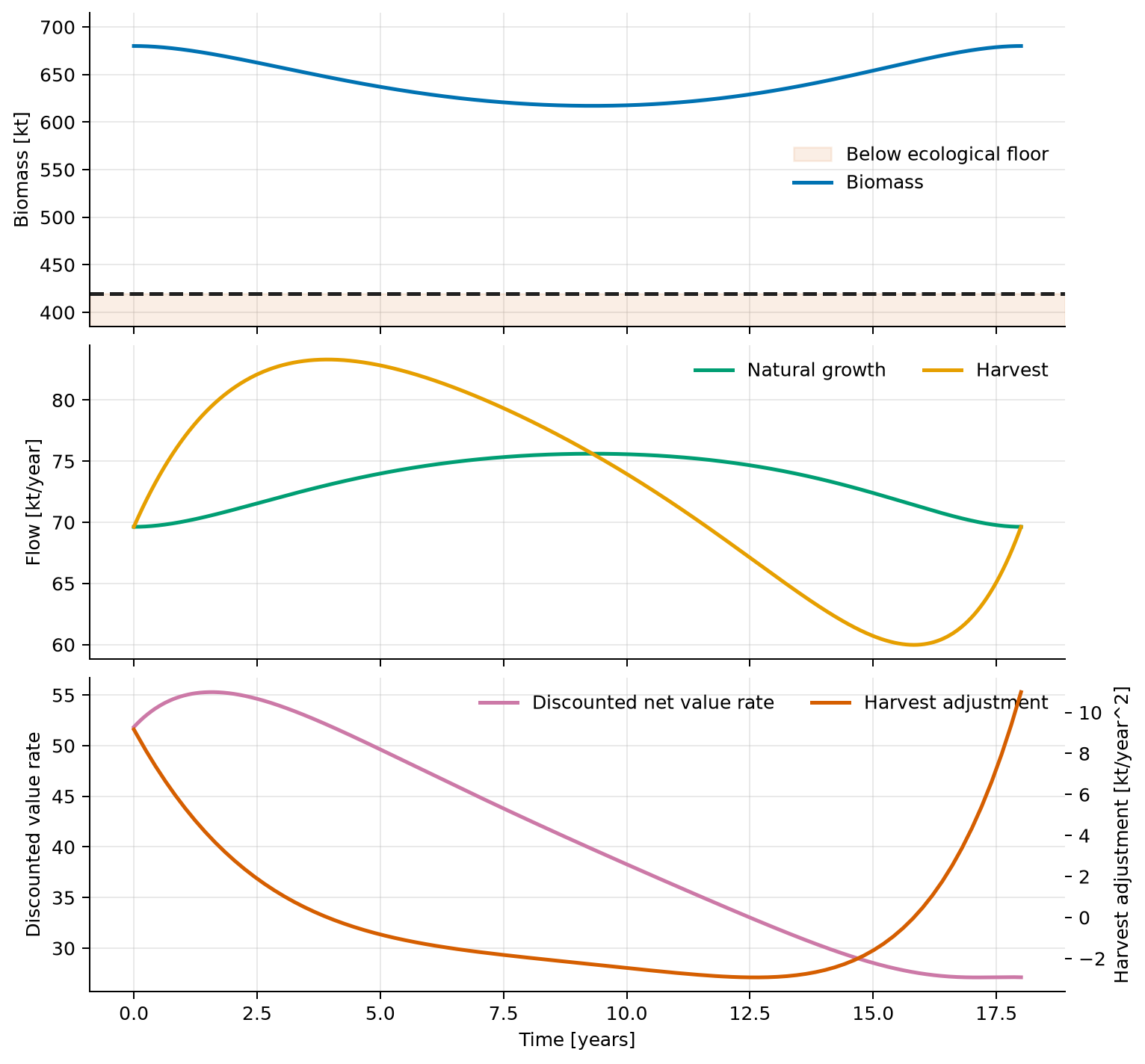
Discounting gives earlier net value more weight. Consequently, even with cyclic endpoints, the optimal policy brings some harvest forward and rebuilds the stock later. The cyclic conditions remove a terminal liquidation incentive; they do not remove this within-horizon timing effect.

The script uses a \(90\times3\) Lobatto discretization and reconstructs the solution at 6,001 times for checks that are independent of the NLP node values.

Independent validation

Integrating the biomass equation gives

\[ B(T)-B(0)=\int_0^T\left[G(B(t))-H(t)\right]\,\mathrm{d}t. \]

Because \(B(T)=B(0)\), cumulative harvest must equal cumulative natural production. The script evaluates this identity with dense-grid trapezoidal quadrature. It similarly checks

\[ H(T)-H(0)=\int_0^T u(t)\,\mathrm dt=0. \]

It also recomputes discounted net value directly from the reconstructed trajectory and compares it with the optimizer objective.

Verified result

Quantity	Verified value
Discounted net value \(V\)	\(734.48532130\)
Minimum biomass	\(617.093132\) kt
Peak harvest rate	\(83.313354\) kt/year
Cumulative harvest	\(1318.215811\) kt
Renewable-stock balance error	\(1.174\times10^{-6}\) kt
Dense objective error	\(3.262\times10^{-6}\)
Maximum dense path-bound violation	\(0\)

The ecological floor is inactive in this parameter set: biomass remains about \(197\) kt above it. That is a result of these prices, costs, endpoints, and horizon, not a general guarantee of bioeconomic optimization.

Scope and limitations

This deterministic aggregate model omits age structure, recruitment and weather uncertainty, fleet heterogeneity, price feedback, enforcement, and spatial migration. Discounted cyclic endpoints can produce front-loaded harvest and should not be interpreted as a stationary policy that can be repeated indefinitely. A management study would require calibrated biological and economic data plus uncertainty and robustness analysis.

Run the example

python -m examples.bioeconomic_fishery

Save the figure without opening a window:

python -m examples.bioeconomic_fishery --save bioeconomic-fishery.png --no-show

system, phase = build_problem()
guess = initial_guess(phase)
solution = solve_problem(system, guess)
plot_solution(solution)

Source code

See the complete runnable example: examples/bioeconomic_fishery.py.