Minimum-Fluence Two-Level Quantum State Transfer

Background

A resonantly driven two-level quantum system can be represented by a Bloch vector in the rotating frame. Under the rotating-wave approximation and zero detuning, the effective Rabi controls rotate that vector on the unit sphere. This example transfers the state from the north pole to the positive \(x\)-axis in fixed time while minimizing the integral of the squared Rabi rate, referred to here as normalized Rabi-control fluence.

The optimal trajectory is a great-circle rotation with a known constant control. It therefore tests nonlinear dynamics, terminal equality constraints, control bounds, and preservation of a geometric invariant against an analytical answer.

Problem formulation

Let

\[ \boldsymbol r=(r_x,r_y,r_z)^{\mathsf T}, \qquad \boldsymbol\Omega=(\Omega_x,\Omega_y,0)^{\mathsf T} \]

be the Bloch vector and resonant Rabi angular-frequency control. In the rotating frame, the ideal coherent Bloch equation is

\[ \dot{\boldsymbol r}=\boldsymbol\Omega\times\boldsymbol r, \]

or componentwise

\[ \begin{aligned} \dot r_x&=\Omega_y r_z,\\ \dot r_y&=-\Omega_x r_z,\\ \dot r_z&=\Omega_x r_y-\Omega_y r_x. \end{aligned} \]

The fixed horizon is \(T=2\). The initial and target states are

\[ \boldsymbol r(0)=(0,0,1)^{\mathsf T}, \qquad \boldsymbol r(T)=(1,0,0)^{\mathsf T}. \]

The normalized Rabi-control fluence and componentwise control bounds are

\[ \min_{\boldsymbol r,\boldsymbol\Omega} J=\int_0^T(\Omega_x^2+\Omega_y^2)\,\mathrm dt, \qquad |\Omega_x|,|\Omega_y|\le2. \]

Analytical optimum

The two endpoint vectors are separated by a Bloch-sphere angle \(\pi/2\). Because \(\lVert\dot{\boldsymbol r}\rVert\le \lVert\boldsymbol\Omega\rVert\), every feasible pulse satisfies

\[ \int_0^T\lVert\boldsymbol\Omega\rVert\,\mathrm dt\ge\frac{\pi}{2}. \]

Cauchy-Schwarz then gives the lower bound

\[ J\ge\frac{1}{T} \left(\int_0^T\lVert\boldsymbol\Omega\rVert\,\mathrm dt\right)^2 \ge\frac{\pi^2}{4T}. \]

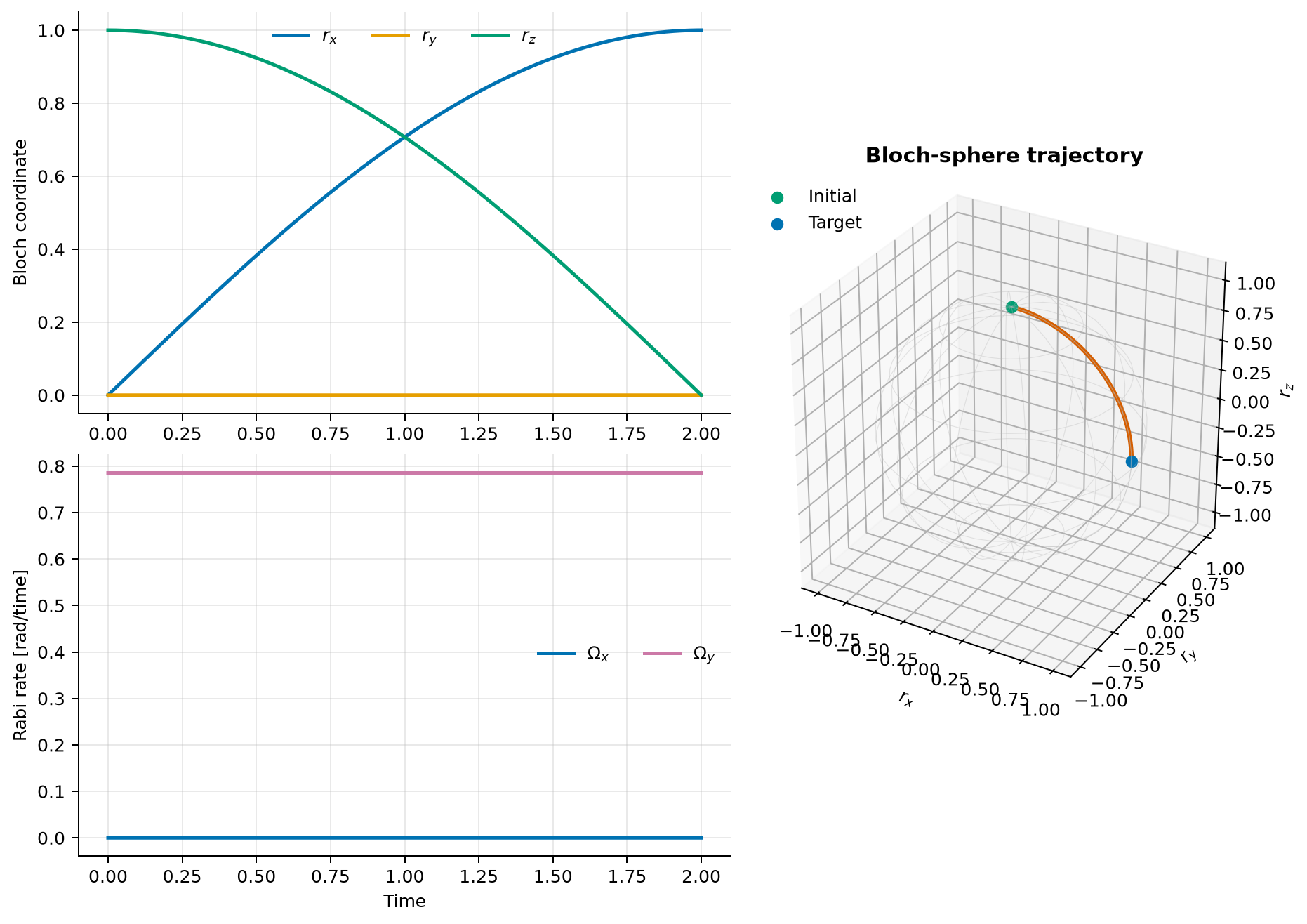
Equality is attained by the constant \(y\)-axis pulse

\[ \Omega_x^*(t)=0, \qquad \Omega_y^*(t)=\frac{\pi}{2T}=\frac{\pi}{4}, \]

which produces

\[ \boldsymbol r^*(t)= \left( \sin\frac{\pi t}{2T}, 0, \cos\frac{\pi t}{2T} \right)^{\mathsf T}. \]

Thus \(J^*=\pi^2/(4T)=\pi^2/8\). The control bound is inactive because \(\pi/4<2\).

Variables and units

Symbol	Meaning	Unit
\(t\)	Scaled time	time unit
\(r_x,r_y,r_z\)	Bloch-vector coordinates	dimensionless
\(\Omega_x,\Omega_y\)	Resonant Rabi rates	rad/time unit
\(J\)	Normalized Rabi-control fluence	rad²/time unit
\(F\)	Pure-state terminal fidelity	dimensionless

Modeling choices

The Bloch equation preserves the sphere automatically:

\[ \frac{\mathrm d}{\mathrm dt}\lVert\boldsymbol r\rVert_2^2 =2\boldsymbol r^{\mathsf T} (\boldsymbol\Omega\times\boldsymbol r)=0. \]

The transcription therefore does not add a redundant unit-norm path constraint. Instead, the script reconstructs the trajectory densely and reports its norm drift. Terminal fidelity is evaluated as

\[ F=\frac{1+\boldsymbol r_{\mathrm{target}}^{\mathsf T}\boldsymbol r(T)}{2}. \]

A \(24\times4\) Lobatto mesh resolves the smooth great-circle trajectory. The exact constant-pulse solution is also used as the initial guess, making this example a validation benchmark rather than a difficult globalization test.

The model assumes exact resonance, the rotating-wave approximation, and coherent closed-system dynamics. It neglects detuning, calibration error, bandwidth, relaxation, and decoherence. The controls are effective Rabi angular frequencies, not laboratory electric-field amplitudes; consequently \(J\) is a normalized fluence and must not be interpreted or extrapolated as experimental pulse energy in joules.

Run the example

python -m examples.quantum_state_transfer

Save the figure without opening a window:

python -m examples.quantum_state_transfer --save quantum-state-transfer.png --no-show

system, phase = build_problem()
guess = initial_guess(phase)
solution = solve_problem(system, guess)
plot_solution(solution)

Verified result

The numerical state and both controls are reconstructed at 4,001 times. The script checks the control bounds, Bloch norm, objective, control area, and terminal fidelity against the analytical solution.

Quantity	Verified value
Numerical normalized fluence \(J\)	\(1.2337005501\)
Analytical fluence \(\pi^2/8\)	\(1.2337005501\)
\(y\)-axis Rabi-control area	\(1.5707963268\ \mathrm{rad}=\pi/2\)
Terminal fidelity	\(1.0000000000\)
Maximum Bloch-norm error	\(1.910\times10^{-8}\)

The numerical control is the constant analytical control to reported precision, and the reconstructed state follows the expected quarter great circle.

Source code

See the complete runnable example: examples/quantum_state_transfer.py.