Minimum-Time Double Integrator: Mathematical Reference

Background

A double integrator models one-dimensional motion when acceleration is the command. It is small enough to solve analytically, but it still exercises free final time, bounded control, a discontinuous optimum, and dense post-solve validation. Those properties make it a useful reference problem for checking an optimal-control implementation.

This page records the model and its verification contract. For a step-by-step introduction to the Pockit API, start with the Getting Started tutorial.

Mathematical model

A unit mass starts one meter from its target at rest. Position \(x\) is measured relative to the target, velocity is \(v\), and acceleration \(u\) is bounded by one meter per second squared. The free-final-time problem is

\[ \begin{aligned} \min_{x,v,u,t_f}\quad & J=t_f=\int_0^{t_f}1\,\mathrm dt,\\ \text{subject to}\quad & \dot x=v,\qquad \dot v=u,\\ & x(0)=1,\qquad v(0)=0,\\ & x(t_f)=0,\qquad v(t_f)=0,\\ & -1\le u(t)\le1. \end{aligned} \]

There are no state path constraints. Both endpoint states are fixed, while \(t_f\) is an optimization variable.

Closed-form solution

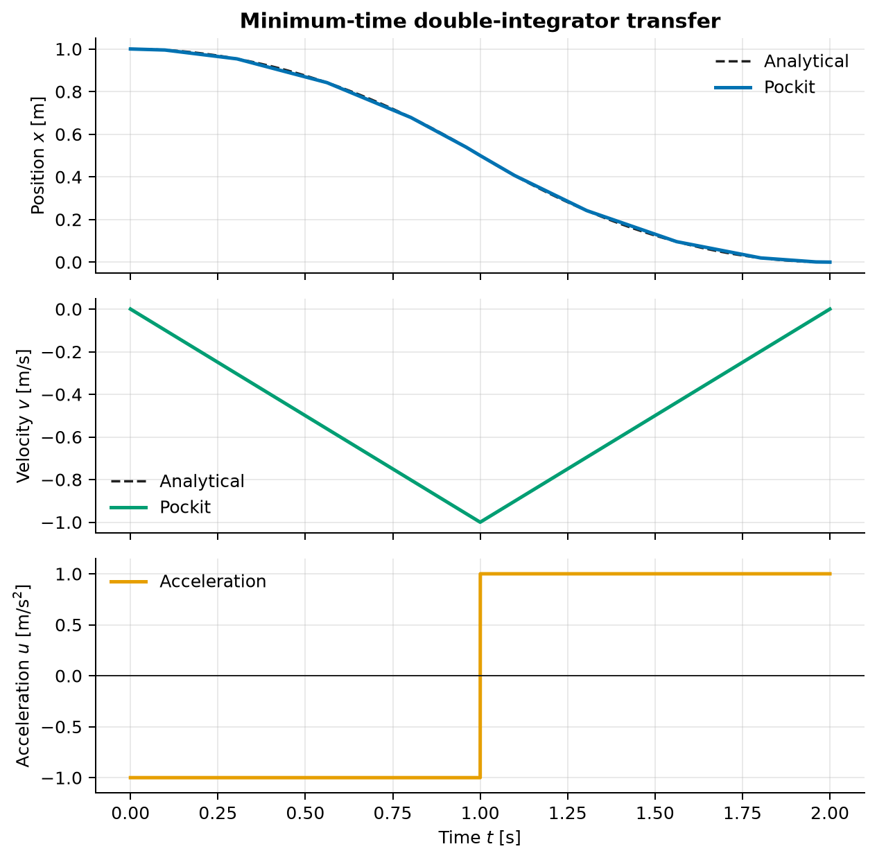
The minimum-time control uses the full available acceleration. It accelerates toward the target for one second and then applies the opposite acceleration to stop:

\[ u^*(t)= \begin{cases} -1, & 0\le t<1,\\ +1, & 1<t\le2. \end{cases} \]

The corresponding state history is

\[ (x^*(t),v^*(t))= \begin{cases} \left(1-\frac12t^2,-t\right), & 0\le t\le1,\\[4pt] \left(\frac12(2-t)^2,t-2\right), & 1\le t\le2. \end{cases} \]

To see why the switching time is one second, let each saturated arc last \(\tau\). The first and second arcs each contribute a displacement of \(-\tau^2/2\), so the total displacement is \(-\tau^2=-1\). Hence \(\tau=1\) and \(t_f^*=2\).

This isolated bang-bang switch is not a singular arc: the optimal control is at a bound on each open arc. The singular-arc guide explains the distinction and Pockit's current limitation.

Variables and units

Symbol	Meaning	Unit
\(t\)	Time	s
\(x\)	Position relative to the target	m
\(v\)	Velocity	m/s
\(u\)	Acceleration command	m/s²
\(t_f\)	Free final time	s

Constraints and transcription

The physical control limit is \(\lvert u\rvert\le1\). The numerical model uses the negligible interior limit

\[ \lvert u\rvert\le1-10^{-7} \]

at collocation points. This buffer absorbs nonlinear-programming tolerance so that the reconstructed control remains inside the physical limit. It changes the analytical final time by only about \(10^{-7}\ \mathrm{s}\), which is reported rather than hidden.

The implementation uses two Radau mesh intervals with six collocation points per interval. Their shared boundary is fixed at normalized time \(0.5\), where the analytical control switches. Ipopt is run with bound_relax_factor=0.0 so it does not relax the stated numerical bounds.

Run the example

From the repository root, run:

python -m examples.double_integrator

For a non-interactive run that saves the figure:

python -m examples.double_integrator --save double-integrator.png --no-show

Numerical validation

The script accepts only successful Ipopt termination, checks the terminal position and velocity to an absolute tolerance of \(10^{-7}\), verifies the sign of both control arcs, and reconstructs acceleration at 10,001 uniformly spaced physical times.

The verified solution gives

Quantity	Numerical value	Analytical value
Final time \(t_f\)	\(2.000000100109\ \mathrm{s}\)	\(2\ \mathrm{s}\)
Switching time	\(1.000000050055\ \mathrm{s}\)	\(1\ \mathrm{s}\)
Dense acceleration range	\([-0.999999900154, 0.999999902382]\ \mathrm{m/s^2}\)	\([-1,1]\ \mathrm{m/s^2}\)

The small time difference is consistent with the documented \(10^{-7}\) collocation buffer. The dense control history remains within the physical acceleration bound over the entire phase, not only at collocation nodes.

Source code

See the complete runnable example: examples/double_integrator.py.