Two-Phase Pharmacokinetic Infusion Control

Educational model, not clinical advice

This synthetic example explains optimal-control modeling. Its parameters are not patient-specific; it omits uncertainty, toxicity, covariates, measurement feedback, and clinical monitoring. It must not be used to select or recommend a dose.

Background

After intravenous administration, a compound may exchange between plasma and peripheral tissue before its effect-site concentration catches up with plasma exposure. A practical infusion command should approach the target quickly, but it should also respect exposure limits and avoid instantaneous changes that a pump cannot reproduce.

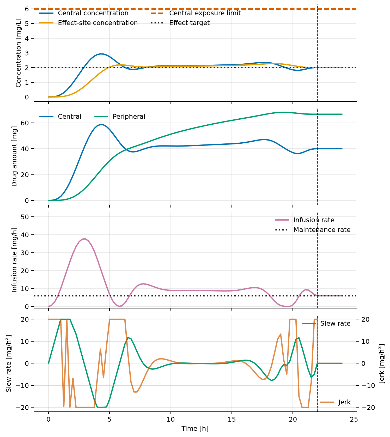
This example separates treatment into two phases. During a 22-hour loading phase, optimization chooses a smooth pump trajectory. During the final two hours, the pump holds the analytically derived maintenance rate and the PK states remain at equilibrium. The split makes the loading-to-maintenance event explicit and demonstrates a biomedical multi-phase model.

Pharmacokinetic model

Let \(A_c\) and \(A_p\) denote drug amounts in the central and peripheral compartments, and let \(C_e\) denote effect-site concentration. Central concentration is

\[ C_c=\frac{A_c}{V_c}. \]

The two-compartment PK model with a first-order effect site is

\[ \begin{aligned} \dot A_c &=R-\left(\frac{CL}{V_c}+k_{12}\right)A_c+k_{21}A_p,\\ \dot A_p&=k_{12}A_c-k_{21}A_p,\\ \dot C_e&=k_{e0}(C_c-C_e), \end{aligned} \]

where \(R\) is the intravenous infusion rate. The effect site is a lagged measurement compartment and does not remove mass from the PK compartments.

Loading phase

On \(0\le t\le t_s=22\ \mathrm{h}\), infusion rate and slew rate are states,

\[ \dot R=S,\qquad \dot S=j, \]

and pump jerk \(j\) is the control. The loading state and control are therefore

\[ \boldsymbol{x}_L=(A_c,A_p,C_e,R,S)^{\mathsf T}, \qquad u_L=j. \]

Starting from a drug-free, stopped pump, the phase must reach the steady maintenance state:

\[ \boldsymbol{x}_L(0)=\boldsymbol{0},\qquad \boldsymbol{x}_L(t_s)= \begin{bmatrix}A_c^*&A_p^*&C^*&R^*&0\end{bmatrix}^{\mathsf T}. \]

For target concentration \(C^*=2\ \mathrm{mg/L}\), mass balance gives

\[ A_c^*=V_cC^*=40\ \mathrm{mg},\qquad A_p^*=\frac{k_{12}}{k_{21}}A_c^*=66.\overline{6}\ \mathrm{mg}, \qquad R^*=CL\,C^*=6\ \mathrm{mg/h}. \]

The loading objective balances tracking and normalized pump effort:

\[ \begin{aligned} J_L=\int_0^{t_s}\Bigg[ &\left(\frac{C_e}{C^*}-1\right)^2 +w_R\left(\frac{R}{R_{\max}}\right)^2\\ &+w_S\left(\frac{S}{S_{\max}}\right)^2 +w_j\left(\frac{j}{j_{\max}}\right)^2 \Bigg]\,\mathrm{d}t, \end{aligned} \]

with \(w_R=0.02\), \(w_S=0.002\), and \(w_j=0.0002\).

Maintenance phase

On \(t_s\le t\le T=24\ \mathrm{h}\), the pump is fixed at \(R^*\). The phase contains only \((A_c,A_p,C_e)\), follows the same PK dynamics, and fixes both endpoints to \((A_c^*,A_p^*,C^*)\). Substitution into the dynamics gives

\[ \dot A_c=\dot A_p=\dot C_e=0, \]

so the maintenance solution is an exact equilibrium rather than a heuristic constant-dose segment. Its contribution to the objective is

\[ J_M=\int_{t_s}^{T} \left[ \left(\frac{C_e}{C^*}-1\right)^2 +w_R\left(\frac{R^*}{R_{\max}}\right)^2 \right]\,\mathrm{d}t, \qquad J=J_L+J_M. \]

Bounds and units

The loading phase enforces

\[ \begin{gathered} A_c\ge0,\qquad 0\le A_p\le200\ \mathrm{mg},\\ 0\le C_e\le4\ \mathrm{mg/L},\qquad C_c\le6\ \mathrm{mg/L},\\ 0\le R\le50\ \mathrm{mg/h},\qquad |S|\le20\ \mathrm{mg/h^2},\qquad |j|\le20\ \mathrm{mg/h^3}. \end{gathered} \]

Symbol	Meaning	Value or unit
\(t\)	Time	h
\(A_c,A_p\)	Central and peripheral amounts	mg
\(C_c,C_e,C^*\)	Central, effect-site, and target concentrations	mg/L
\(R\)	Infusion rate	mg/h
\(S\)	Infusion slew rate	mg/h²
\(j\)	Infusion jerk	mg/h³
\(V_c\)	Central volume	\(20\ \mathrm{L}\)
\(CL\)	Clearance	\(3\ \mathrm{L/h}\)
\(k_{12},k_{21}\)	Inter-compartment rates	\(0.25,0.15\ \mathrm{h^{-1}}\)
\(k_{e0}\)	Effect-site equilibration rate	\(0.50\ \mathrm{h^{-1}}\)

Modeling choices and limitations

Amounts are used as conserved compartment states, while volume converts the central amount to concentration. Promoting \(R\) and \(S\) to states makes the command twice continuously differentiable and lets the model state pump slew and jerk limits directly. The explicit maintenance phase is useful whenever a known operating regime follows a transient optimized regime.

The model assumes linear, time-invariant PK parameters and continuous intravenous delivery. The tracking objective is a numerical teaching device, not a pharmacodynamic benefit or toxicity model. A clinical formulation would need population or patient-specific parameter uncertainty, safety endpoints, sampled feedback, device dynamics, and medical review.

The loading phase uses an \(88\times2\) Lobatto mesh; the maintenance phase uses an \(8\times3\) mesh. A smooth cubic ramp initializes the loading states, slew, and jerk, while the second phase starts from the analytical equilibrium.

Run the example

python -m examples.pharmacokinetic_dosing

Save the figure without opening a window:

python -m examples.pharmacokinetic_dosing --save pharmacokinetic-dosing.png --no-show

The implementation follows the common multi-phase pipeline:

system, phases = build_problem()
guess = initial_guess(phases)
solution = solve_problem(system, guess)
plot_solution(solution)

Verified result

The script reconstructs both phases on one 4,001-point time grid. It checks every state and actuator bound, the terminal target, constancy of the complete maintenance segment, and the terminal PK and pump derivatives.

Quantity	Verified value
Objective \(J\)	\(2.85018982\)
Total administered dose \(\int_0^T R\,\mathrm{d}t\)	\(249.448036\ \mathrm{mg}\)
Effect-site tracking RMSE	\(0.683745\ \mathrm{mg/L}\)
Peak central concentration	\(2.935014\ \mathrm{mg/L}\)
Maximum terminal-state error	\(0\) at printed precision
Maximum maintenance-phase deviation	\(1.421\times10^{-14}\)
Terminal PK/pump equilibrium residual	\(0\) at printed precision
Maximum dense path-bound violation	\(1.906\times10^{-7}\)

The loading trajectory reaches the complete PK and pump equilibrium at \(t_s\), after which the analytical \(6\ \mathrm{mg/h}\) rate holds every reported state constant. The dense path violation remains below the script's \(2\times10^{-6}\) numerical acceptance tolerance.

Source code

See the complete runnable educational example: examples/pharmacokinetic_dosing.py.